Notes for Prof. Hung-Yi Lee's ML Lecture: Reinforcement Learning
Overview of Reinforcement Learning
Scenarios
We are training agents. The agents have observations to the environment and then take actions. the action change the environments, and then the environments give the agents rewards. The agents are then udpated based on the rewards.
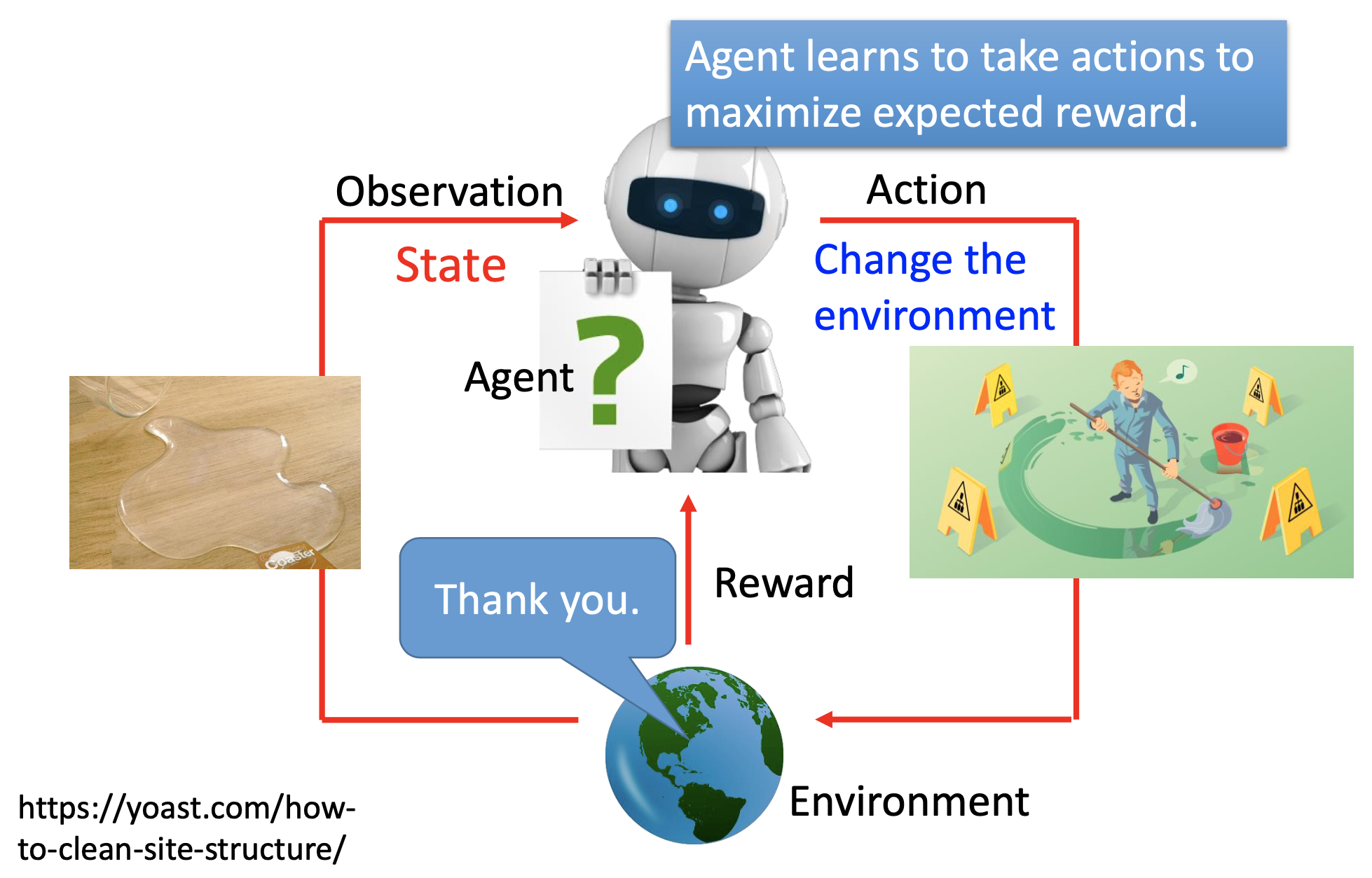
In old days, the models are weaker, so people process the observations into states before feed them to the model. Now the 2 terms observation and state are exchangable.
Comparing Reinforcement Learning & Supervised Learning
A key difference between supervised learning (classification or regression) and reinfrocement learning: in reinforcement learning, the machines’ decision at the current step effect the data (i.e. the environment) of the later steps. In supervised learning, the data is independent from the machines’ current decision.
When we want machines to learn complex behaviors, a problem of behavior cloning, i.e. supervised learning, is that the examples provided by human may include useless movements. By behavior cloning, the machines mimic all the behaviors and cannot recognize which movements are important and which are useless. In the worst cases, the machines may learn only the useless parts and we get poor results. Reinforcement learning can avoid such problem.
Also, in some cases, even we don’t know what are the correct behaviors and cannot provide examples to the machines. Reinforcement learning is suitable for such kind of tasks.
Difficulty of Reinforcement Learning
The reward may be sparse, e.g. in Go, there’s reward only at the end of a game.
Approaches of Reinforcement Learning
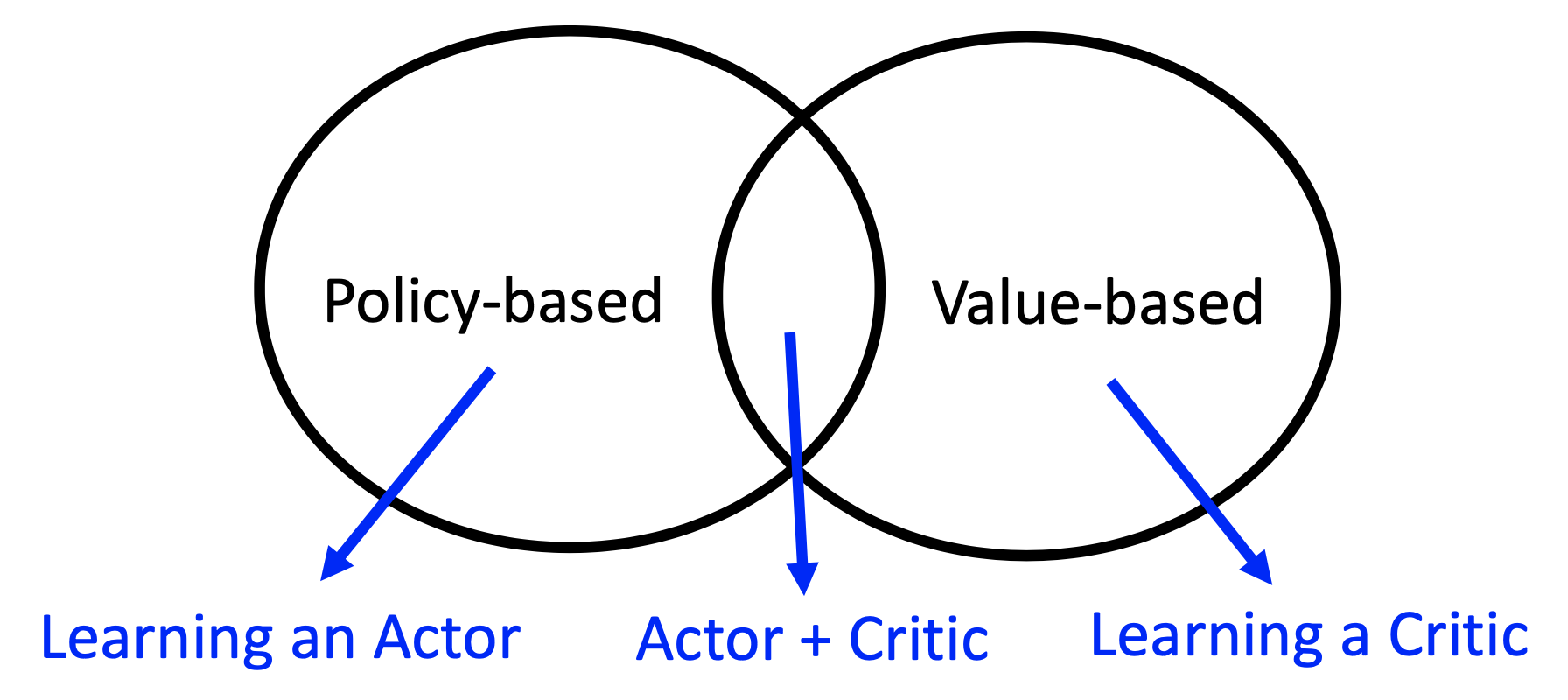
Policy-based: learning an actor. Value-based: learning a critic. A critic evaluates the goodness of states or actions of states.
Learning by Demonstration
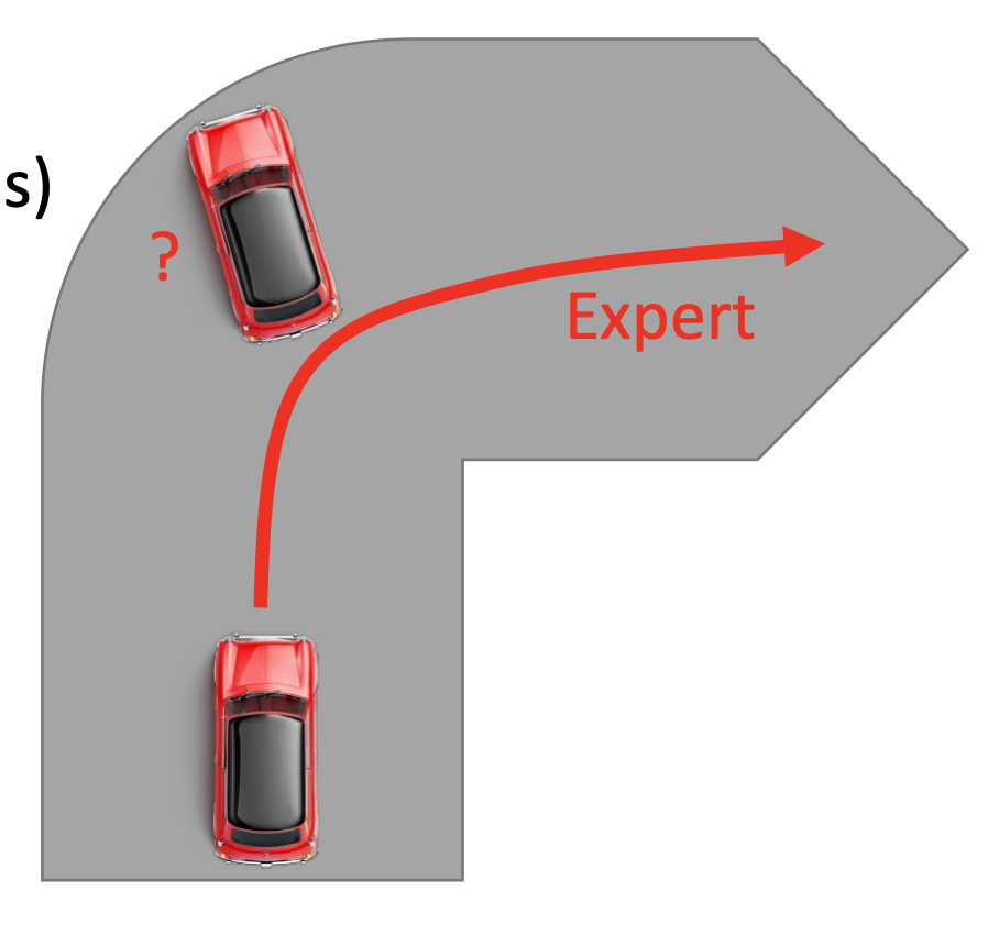
Also imitation learning or apprenticeship learning. An expert demonstrate how to solve the task, and the machine learns from the demonstration. Not behavior cloning! Inverse reinforcement learning is an example.
Comparing Inverse Reinforcement Learning & Behavior Cloning
In supervised learning, we expect training and testing data have the same distribution. But for learning complex behavior, the 2 distribution may vary a lot. IRL can overcome such problem by learning the reward function.
Policy-Based
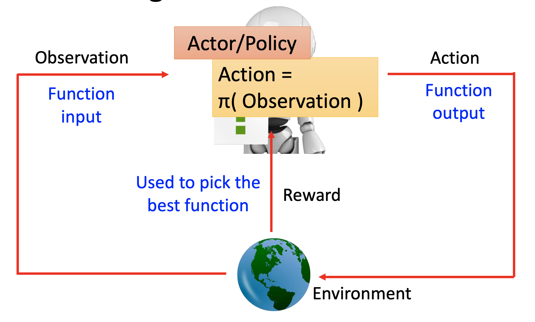
By the policy-based approaches, we are learning actors $\pi$, which are functions that $\pi(observation) = action$. In the mean time, we use the reward from the environment to find the best function.
ML Step 1: Defining a Function Set
For depp reinforcement learning, we use neural networkd as actors. We define the output as the probabilities of the actions. Letting the actor be stochastic may benefit the training because the randomness can let it perform more different trials.
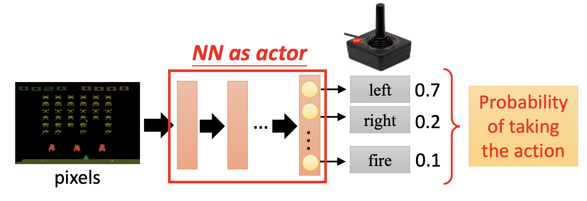
By the old reinforcement learning, we use lookup tables. However, in many cases, we cannot exhaust all the possibility of the observation. We need neural networks’ power of generalization.
ML Step 2: Defining Goodness of functions
We have an actor $\pi_{\theta}(s)$ where $\theta$ represent the parameters of the NN and $s$ in the input observations. When we use the actor $\pi_{\theta}(s)$ to perform the task, at every step $t$, we have observation $s_t$, the actor produce action $a_t$, and the environment provide reward $r_t$. Letting the actor perform the task 1 time is an episode. An episode has a trakectory
\[\tau = \{ s_1, a_1, r_1, \dotsc, s_T, a_T, r_T \}\]and a total reward
\[R(\tau) = \sum_{t=1}^T r_t\]The expected value of total reward over parameter $\theta$ over all possible trajectories is then
\[\overline{R_{\theta}} = \sum_{\tau} R(\tau) P(\tau \vert \theta) \approx \frac{1}{N} \sum_{n=1}^{N} R(\tau^n)\]Where $N$ is the total times we use $\pi_{\theta}$ to perform the task. We then use $\overline{R_{\theta}}$ as the goodness of the actor function.
ML Step 3: Finding the Best Function
We want to find the $\theta$ that maximize the expected reward
\[\theta^* = arg \max\limits_{\theta} \overline{R_{\theta}}\]By gradient ascent,
\[\theta^{new} \gets \theta^{old} + \eta \nabla \overline{R_{\theta^{old}}}\]after some derivation, we get
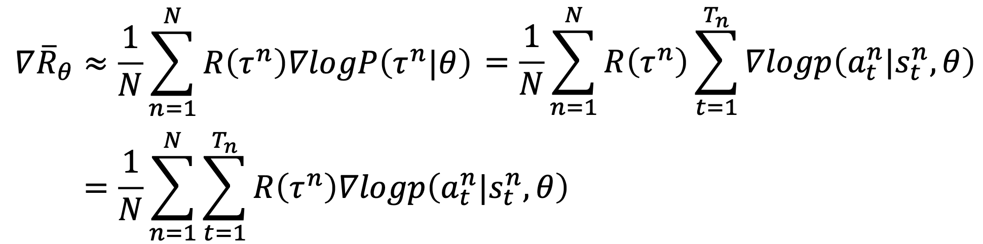
Furthermore, it’s possible that $R(\tau^n)$ is always possitive. In the ideal cases, it’s not a problem. After an update, the probability of the action with the less positive update will actually decrease. However, in practical cases, we samples over the actions, and some actions may never be sampled. If all the $R(\tau^n)$s are positive, the unsampled actions will definitely decrease, and the machine may never try such actions and that may be a unwanted results.
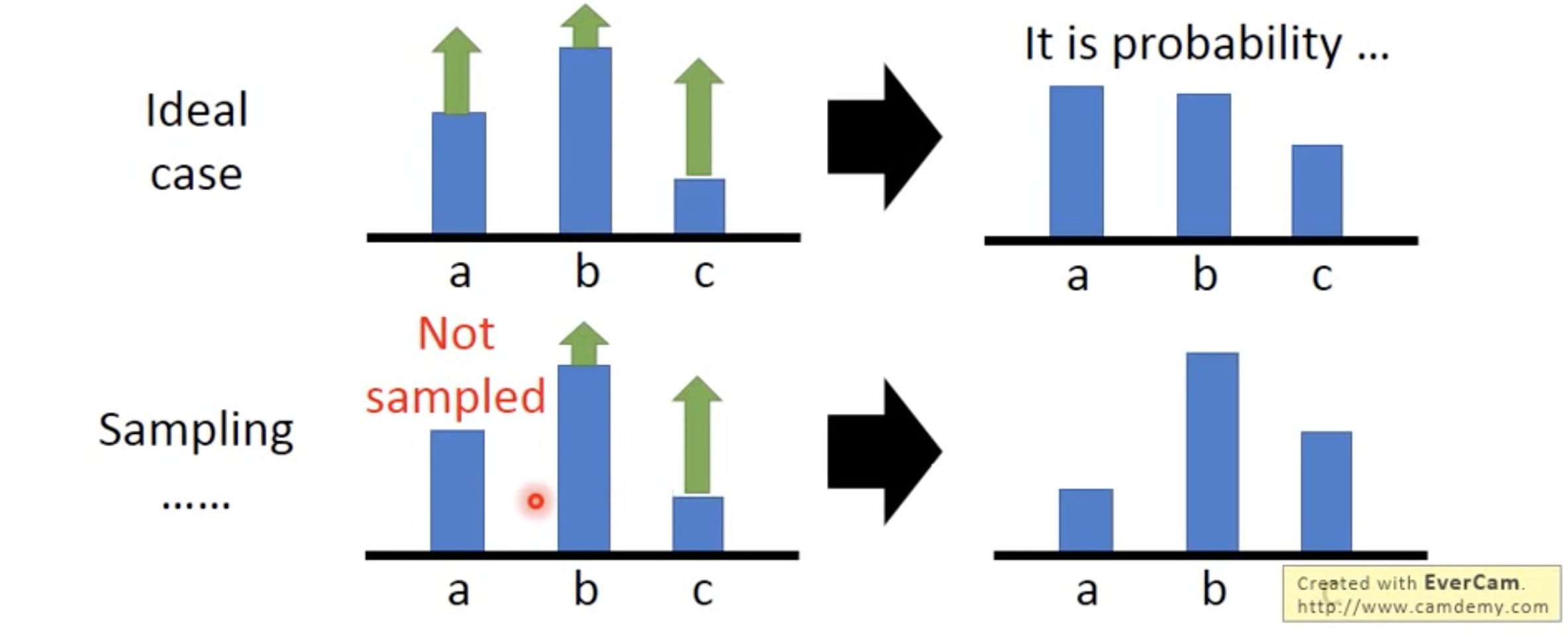
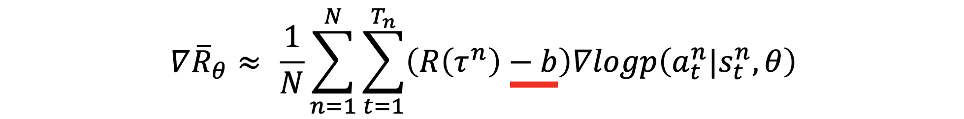
To have more effective plus / minus values of the updates, we subtract a baseline $b$:
Discussion: Using Total Reward
In the gradient ascent, we use $R(\tau^n)$ rather than $r^n_t$ at each single step. It is very important to consider the cumulative reward $R(\tau^n)$ of the whole trajectory $\tau^n$ instead of immediate reward $r^n_t$.
Discussion: Meaning of the Gradient Term
\[\nabla logp(a^n_t \vert s^n_t, \theta) = \frac{\nabla p(a^n_t \vert s^n_t, \theta)}{p(a^n_t \vert s^n_t, \theta)}\]The denomibator is actually reasonable. The actions with high probabilities may be sampled for more times, so they may be updated more after gradient ascent and get even higher probilities. The denominator balanced such effect.
We can also simply see the $logp(a^n_t \vert s^n_t, \theta)$ as a loss function of cross entropy the actual action and its probability. Therefore, the updates over every steps are simply enhancement or reduction of the actual action, while the sign is decided by the total reward and the bias.
Prof. Hung-Yi Lee’s Magic Tip for Deep Learning
“Whenever you find something undifferentiable, train it by policy gradient.”
Value-Based
By value-based approaches, we’re learning critics. A critic does not directly determine the action. Given an actor $\pi$, it evaluates how good the actor is. The output values of a critic depend on the actor evaluated.
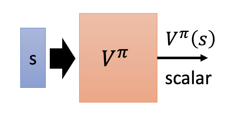
State Value Function $V^{\pi}(s)$
A state value function $V^{\pi}(s)$ output the culmulated reward $G$ obtained after seeing state $s$ by letting actor $\pi$ perform the task.
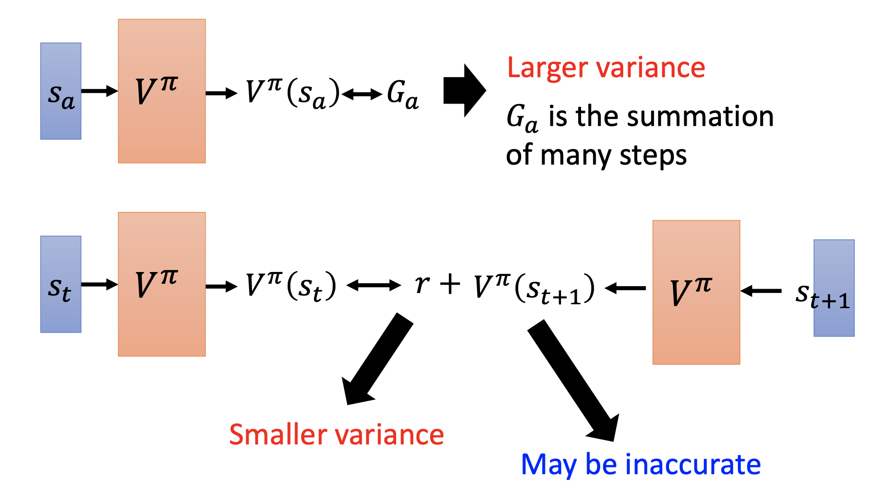
Training $V^{\pi}(s)$
Monte-Carlo (MC) based approach: Use the cumulated reward from seeing $s$ to the end of an episode directly.
Temporal-difference (TD) approach: Use the reward obtained at step $t$ as the difference between $V^{\pi}(s_{t})$ and $V^{\pi}(s_{t+1})$.
Some applications have very long episodes, so that delaying all learning until an episode’s end is too slow and TD may be a better choice.
State-action value function $Q^{\pi}(s, a)$
State-action value function output the cumulated reward expected to be obtained after taking action $a$ at state $s$ when using actor $\pi$.
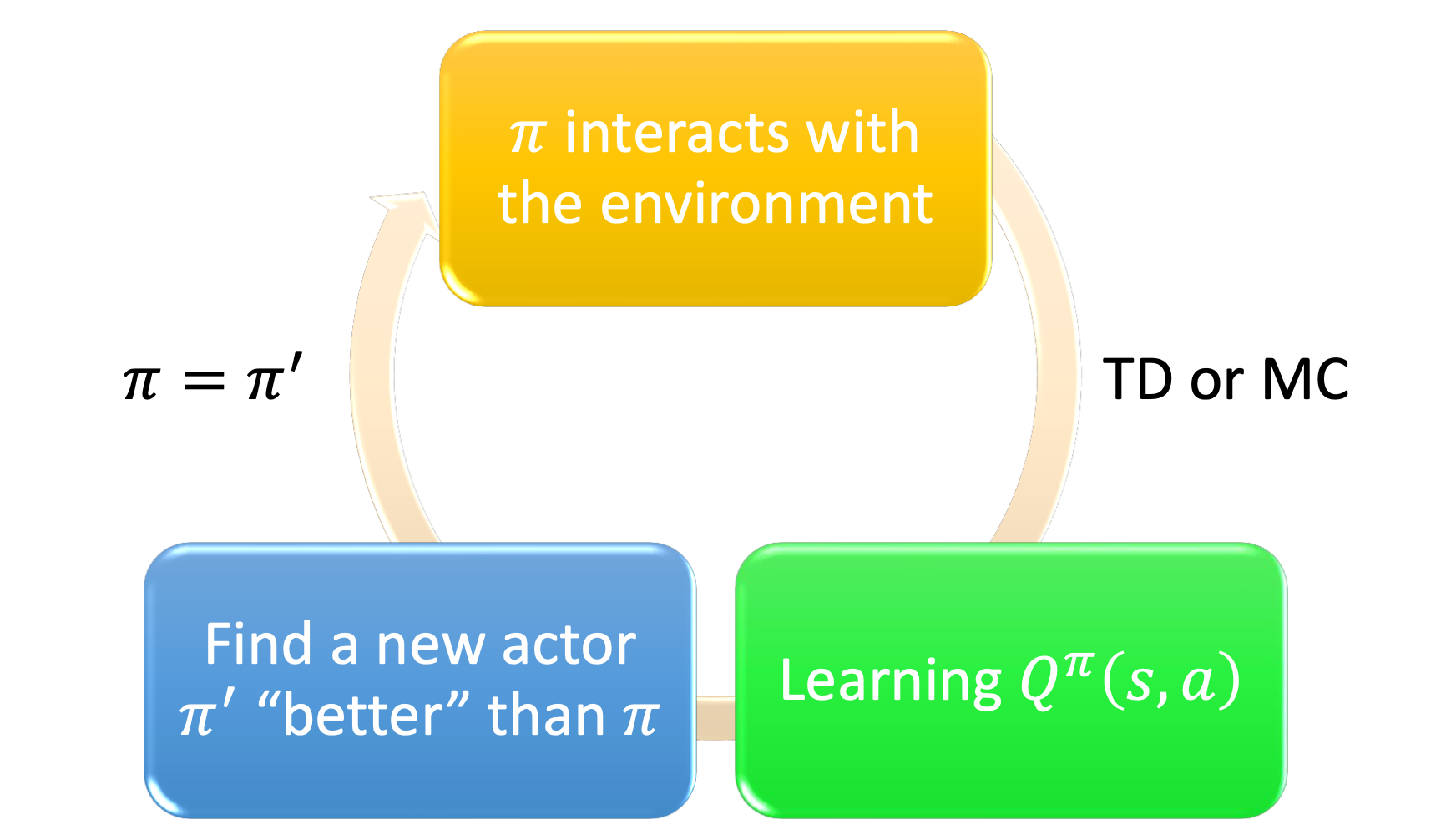
Given $Q^{\pi}(s, a)$, find a new actor $\pi’$ that’s better than $pi$:
\[V^{\pi'}(s) \leq V^{\pi}(s) \text{, } \forall s \\ \pi'(s) = arg \max\limits_{a} Q^{\pi}(s,a)\]For the tricks of Q-learning, google the paper “rainbow”.
Actor-Critic
Concerning that the environment and the reward may vary wildly, we let the actor learn from the critic.
Asynchronous Advantage Actor-Critc: Asynchronous is simply parallelly running many episodes. It has good performance.
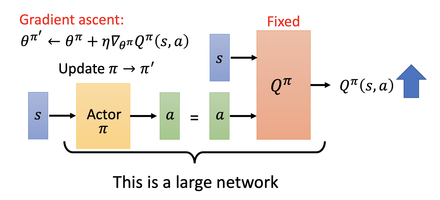
Pathwise Derivative Policy Gradient: Let the actor learn to produce the action $a$ that maximize $Q^{\pi}$. Conceptually similar to GAN.
Inverse Reinforcement Learning
In many applications, it’s difficult to define reward function. Moreover, illy defined reward functions may produce terrible actors.
By inverse reinforcement learning, we use the examples provided by expert to find reward functions, then we use the reward functions to train actors.
Steps of IRL:
- Collect example episodes from the experts.
- Let the actor generate episodes.
- Train the reward function so that it give higher scores to the experts’ episodes than the actors’ episodes.
- Use the trained reward function to get a new actor.
- Repeat from 2 to 4.
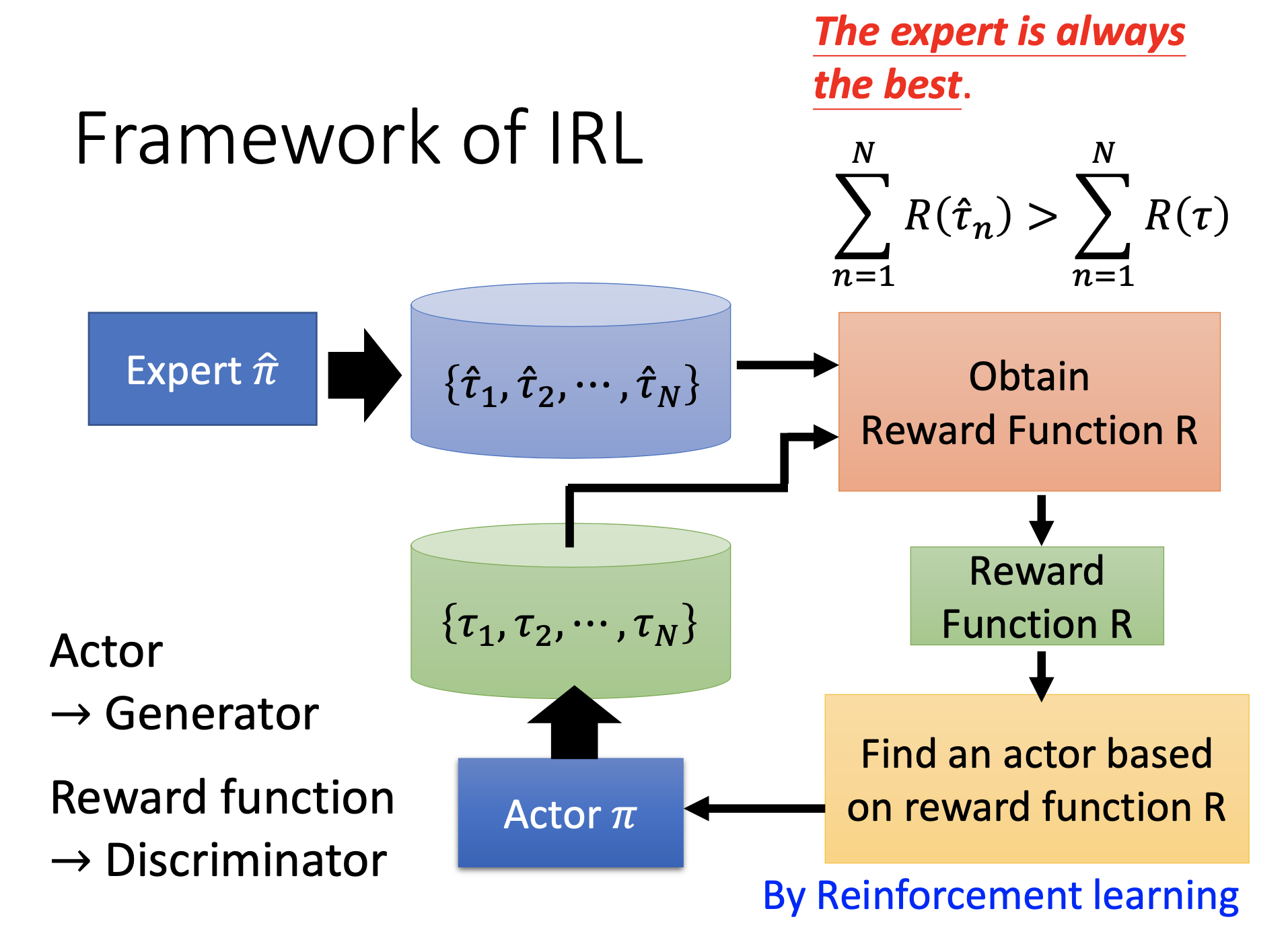
Such process is very similar to GAN.
My Discussion: Comparing with Behavior Cloning
Do the machines copy the useless movements by IRL? I think IRL doesn’t guarantee avoiding such problem.
References
Youtube ML Lecture 23-1: Deep Reinforcement Learning
Youtube ML Lecture 23-2: Policy Gradient (Supplementary Explanation)
Youtube ML Lecture 23-3: Reinforcement Learning (including Q-learning)