Notes for Prof. Hung-Yi Lee's ML Lecture 15: Neighbor Embedding
Manifold Learning
In some data set, it may be meaningless to compute the Euclidean distance directly, especially when the distance between examples are not small. Therefore, in such cases, if we want to perform dimension reduction, it has to be non-linear. Such dimension reduction may benefits for further clustering or supervised learning.
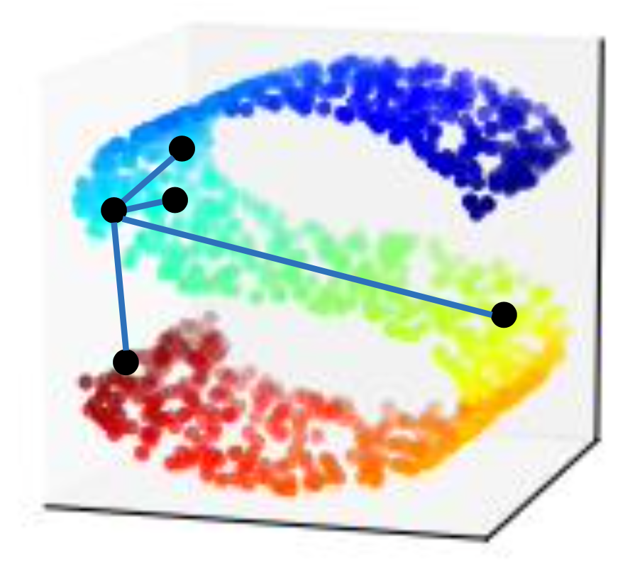
Locally Linear Embedding
「在天願做比翼鳥 在地願為連理枝」
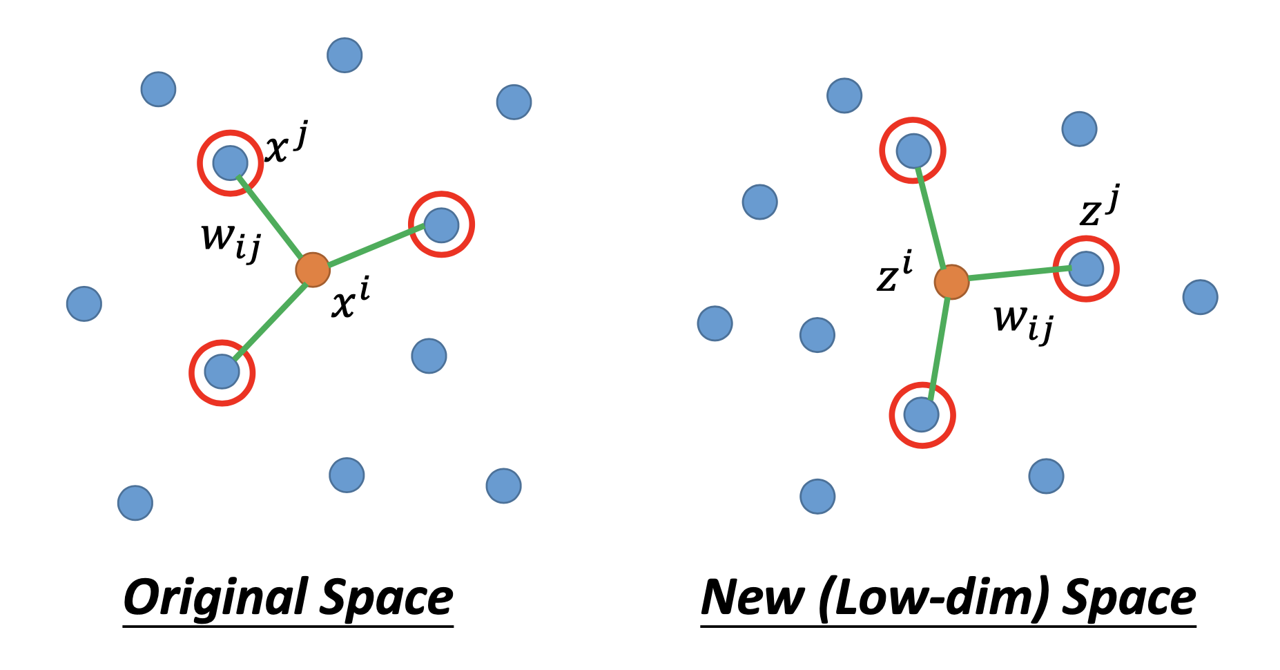
In the original space of $x$, we find $w_{ij}$ for all the examples $x^i$, where $w_{ij}$ represents the relation between $x^i$ and its neighboring points $x^j$s, and $w_{ij}$ miimize
\[\sum_{i} \vert \vert x^i - \sum_j w_{ij} x^j \vert \vert _2\]then we find the dimension reduction results $z^i$ and $z^j$ by minimizing
\[\sum_{i} \vert \vert z^i - \sum_j w_{ij} z^j \vert \vert _2\]so that we can keep $w_{ij}$ unchanged in the new space.
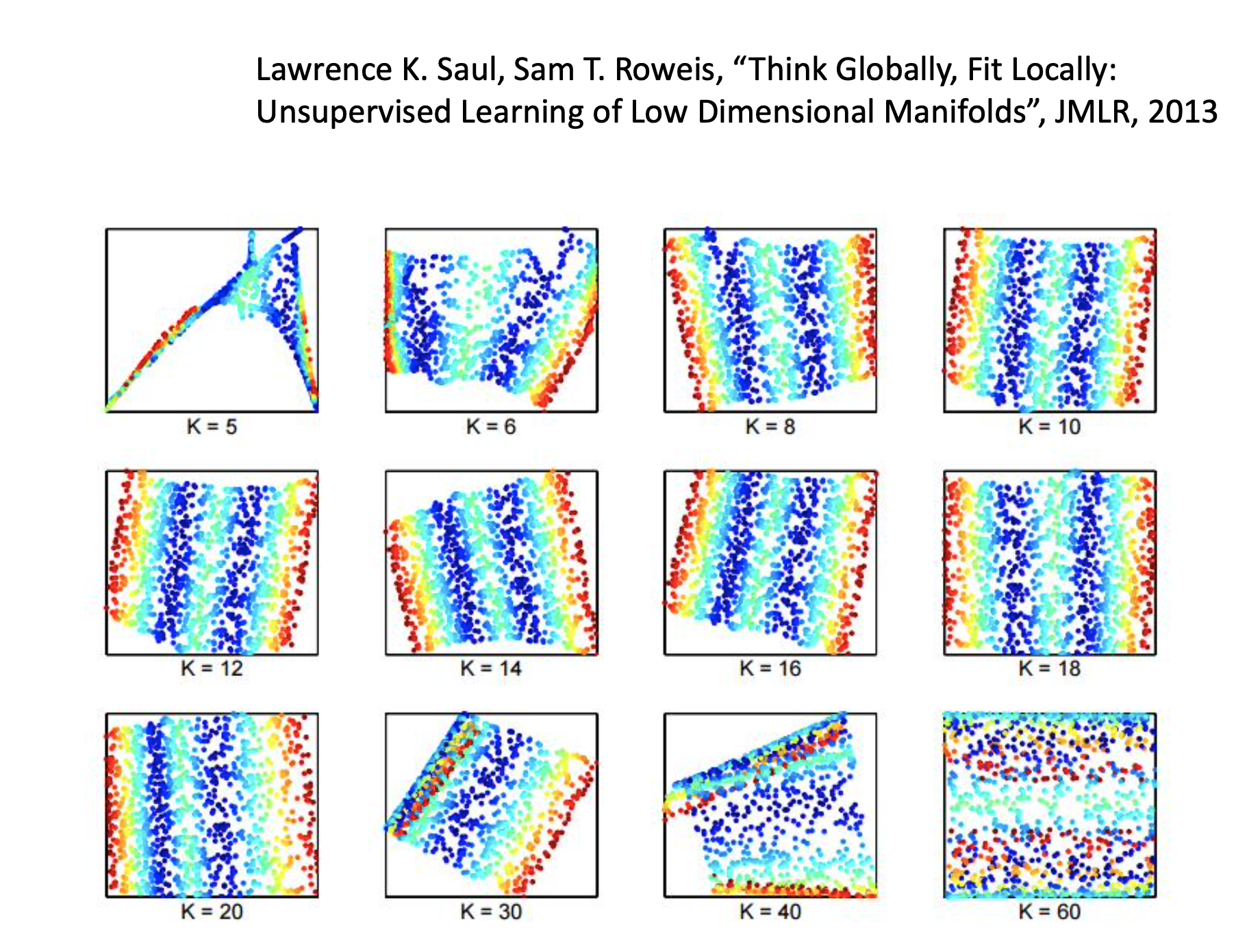
Besides, choosing the number of neighbors is important. By too many neighbors, some of them may be too far to keep the localness so their $w_{ij}$s become meaningless. (I guess) By too few neighbors, the $w_{ij}$s cannot properly describe the relationships between examples.
One advantage of LLE is that, even we don’t have $x$s, we can find $z$s if we have $x$s’ relationships $w_{ij}$.
Since LLE only cares about the neighbors of an example, when adding new data, it should be reasonable to compute only the $z$s without re-computing $z$s of the whole data set.
Laplacian Eigenmaps
We use distance defined by graph approximate the distance on manifold.
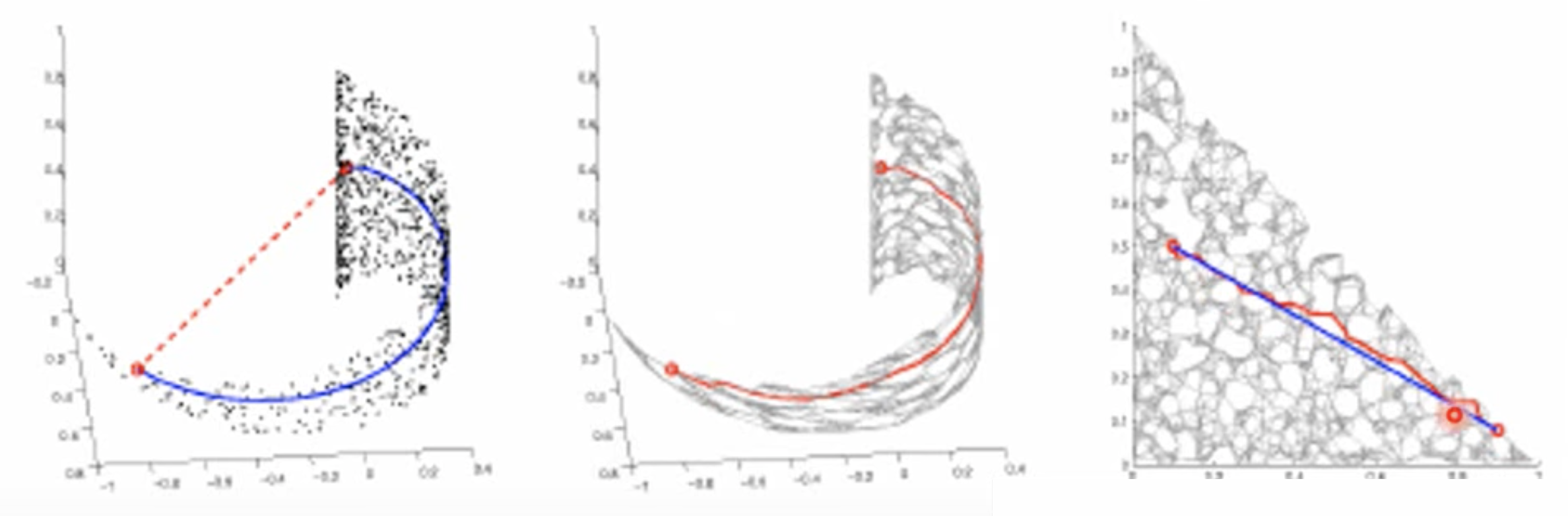
First, we connect the graph and then calculate the similarity
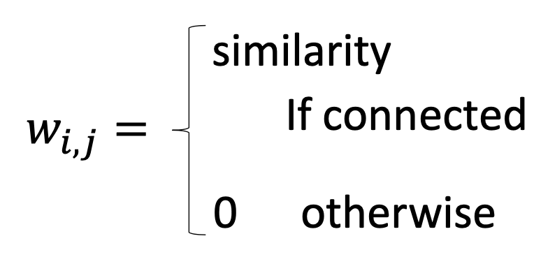
then in the new space of $z$, we find $z$s to minimize
\[S = \frac{1}{2} \sum_{i,j} w_{i,j} \vert \vert z^i - z^j \vert \vert _2\]then $z^1$ and $z2$ will be close to each other if $x1$ and $x2$ are close in a high density region. To avoid the trivial solution that all $z = 0$, we make a further constraint
\[\text{If the dim of } z \text{ is M, } Span \{ z^1, z^2, \dots, z^n \} = R^M\]The solution is the eigenvectors of the graph Laplacian.
Also, Spectral clustering is peforming Laplacian Eigenmaps and then performing clustering.
When adding new examples, it should be ok to compute $z$s for only the new examples, so Laplacian eiganmaps can be used for the training / testing scenarios.
The Problem of Aggregating Clusters
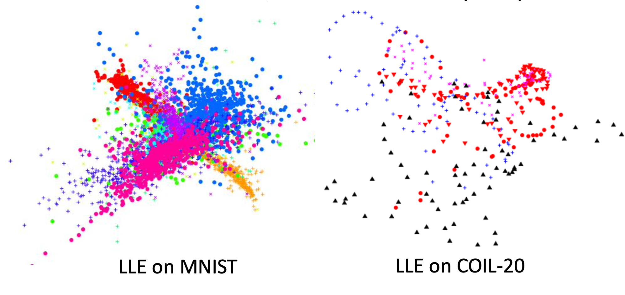
Both LLE and Laplacian eiganmaps have the problem that the non-similar data may also aggregate together because only the relationships between the similar examples are defined. T-SNE can fix this problem.
T-distribution Stochastic Neighboring Embedding
Compute similarity between all pairs of $x: S(x^i,x^j)$, then calculate
\[P(x^j \vert x^i) = \frac{S(x^i, x^j)}{\sum_{k \neq i} S(x^i, x^k)}\]then compute similarity between all pairs of $z: S’(z^i,z^j)$, then calculate
\[P(z^j | z^i) = \frac{S'(z^i, z^j)}{\sum_{k \neq i} S'(z^i, z^k)}\]then find a set of z to minimize the KL entropy
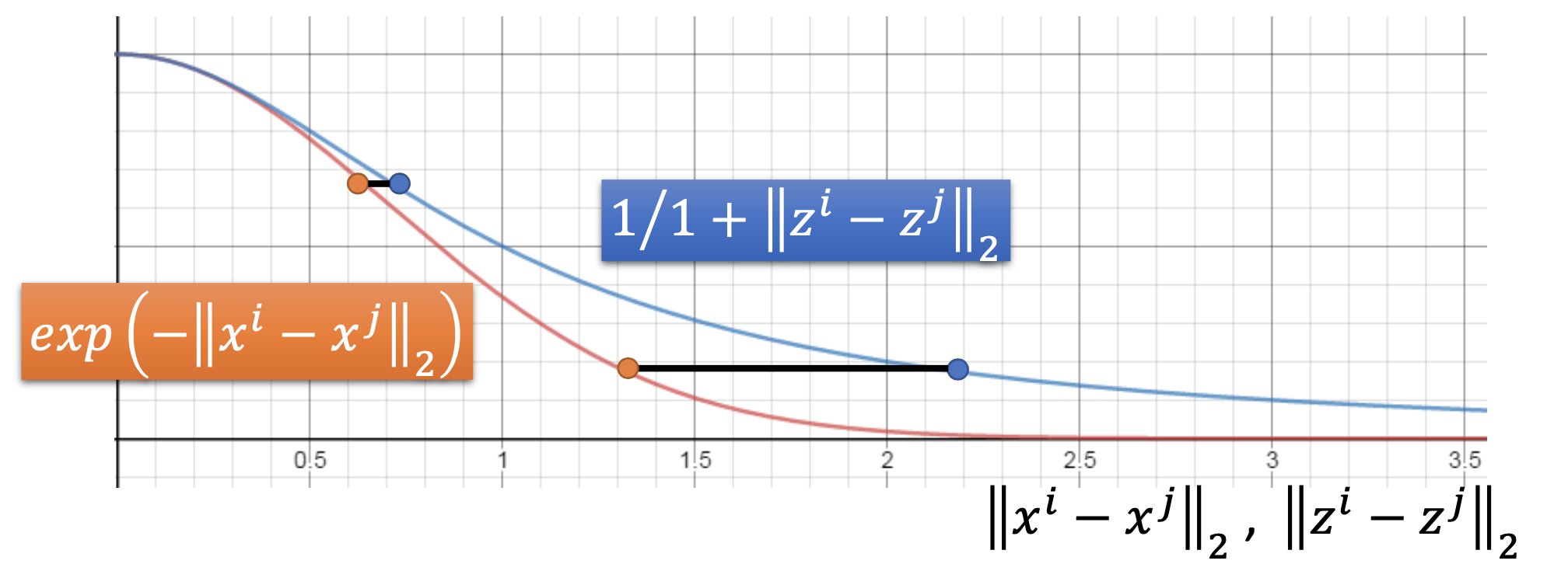
\[L = \sum_{i} KL(P(*|x^i)||Q(*|z^i)) \\ = \sum_{i,j} P(x^j | x^i)log \frac{P(x^j | x^i)}{Q(z^j|z^i)}\]where $S(x^i,x^j) = exp(- \vert \vert x^i - x^j \vert \vert _2)$. For $S’(z^i,z^j)$, in SNE
\[S'(z^i,z^j) = exp(- \vert \vert z^i - z^j \vert \vert _2)\]in T-SNE,
| $S’(z^i,z^j) = \frac{1}{1 + | z^i - z^j | _2}$ |
with the T-distribution, the distance in the space of $x$ will be enlarged in the space of $x$.
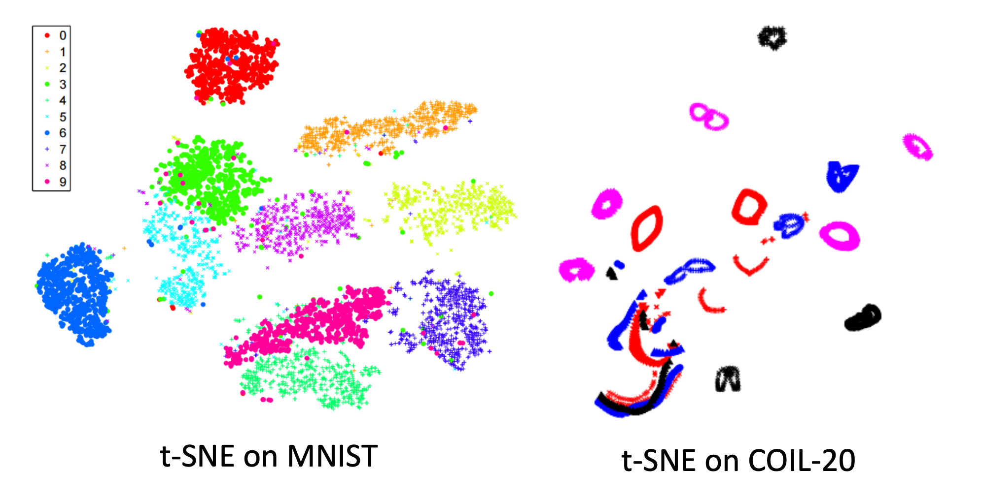
T-SNE can provide very good visualization. In practical scenarios, we often use simple PCA first to reduce the dimensionality once and then use T-SNE to reduce computing cost.
By T-SNE, we have to calculate the KL-divergence for the whole data set, so we have to re-compute the whole transformation once we want to include more data. Therefore, T-SNE is not suitable for the scenarios of training and testing.
My question for adding new data with T-SNE: why not compute only the newly generated probabilities? It seems that we can do it, so it should be not so problematic for computing cost when adding new data. By doing so, the transofrmation of the old examples effect those of the new examples significantly, so we should still re-compute the transformation for the whole old and new data if the amount of the new data is not relatively small to the old.
References
Youtube ML Lecture 15: Unsupervised Learning - Neighbor Embedding