Notes for Prof. Hung-Yi Lee's ML Lecture 12: Semi-Supervised Learning
In supervised learning, all the training data are labelled, i.e. we have
\[\{(x^r, \hat{y}^r)\}^{R}_{r=1}\]While in some scenarios, collecting data is easy but collecting labelled data is expensive, so we may have some labelled data and many unlabelled data, i.e. we have
\[\{(x^r, \hat{y}^r)\}^{R}_{r=1}, \{ x^u \}^{R+U}_{u=R+1}\]Further more, transductive learning is the case that unlabeled data is the testing data, i.e. trying to be sepcific on the problem / task, and inductive learning unlabeled data is not the testing data, i.e. trying to be general.
Semi-Supervised Learning for Generative Models
Steps
Consider a binary classifgication,
Step 0
Initialze the model by the labelled data as in supervised learning:
\[\theta = \{ P(C_1), P(C_2), \mu^1, \mu^2, \Sigma \}\]Step 1
Compute the posterior probability of all the unlabeled data $P_{\theta}(C_1 \vert x^u)$ by the calculated $\theta$.
Step 2
Update the model $\theta$ by
\[P(C_1) = \frac{N_1 + \sum_{x^u} P(C_1 \vert x^u)}{N_{tot}}\] \[\mu^1 = \frac{1}{N_1} \sum_{x^r \in C_1} x^r + \frac{1}{ \sum_{x^u}P(C_1 \vert x^u) } \sum_{x^u}P(C_1 \vert x^u) \dots\]and then repeat from step 1 until $\theta$ converges. $N_{tot}$ is the total number of examples, $N_1$ is the number of examples belonging to $C1$.
Explanation
We are finding the maximum likelihood with labelled data and unlabelled data
\[lnL(\theta) = \sum_{x^r} ln P_{\theta}(x^r, \hat{y}^r) + \sum_{x^u} lnP_{\theta}(x^u)\]while it’s non-convex, so we perform a EM algorithm to solve it iteratively, where
\[P_{\theta}(x^u) = P_{\theta}(x^u \vert C_1)P(C_1) + P_{\theta}(x^u \vert C_2)P(C_2)\]here the labels we make on the originally unlabelled data are soft labels, i.e. an example belong to the classes by probability.
Low Density Seperation Assumption
非黑即白。”It’s either black or white.”
We assume that at the boundary of classes, the density of examples are relatively low.
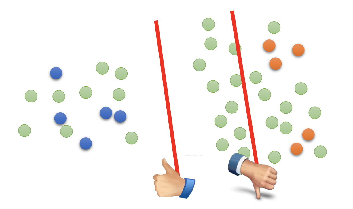
Self-Training
Using the labelled data to train the model first, and then apply the model to the unlabelled data to get more labelled data for further iterative training.
Self-training is a general methodology, so it can be used on any kind of models.
(My argument) By the low density assumption, the boundaries between classes made by the model trained by the labelled data should at least cross some of the low density region, so the model should at least correctly classify some unlabelled data. By choosing the correctly classified unbelled data with some criteria and add them into to labelled data and repeat such processes, we should be able to gradually enlarge the labelled data set and improve the performance of the model.
Steps
Given labelled data set
\[\{(x^r, \hat{y}^r)\}^{R}_{r=1}\]and unlabelled data set
\[\{ x^u \}^{R+U}_{u=R+1}\]Repeat the following steps:
- Train model $f^*$ from labelled data set.
- Apply $f^*$ to the unlabelled data set to get pseudo labels.
- Remove a set of data from unlabeled data set, and add them into the labeled data set.
In step 3, how to choose the data set remains open. You can also provide a weight to each data.
Discussions
Self-training is useless on regression because there will be no error from the $y^u$ generated by $f^*$ and $x^u$. By the same reason, when using self-training on neural networks, we must use hard label.
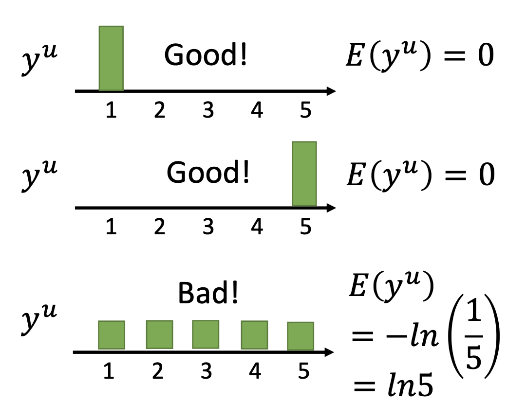
Entropy-Based Regularization
(My argement) By low density separation approximation, most examples should belong to a class with high probability and to other classes with low probality, so the entropy should be low for a successful classifier.
By entropy-based regularization, we minimize the loss function
\[L = \sum_{x^r} C(x^r, \hat{y}^r) + \lambda \sum_{x^u}E(y^u)\]where $C$ is cross entropy and $E$ is the entropy of the predictions on the unlabelled data
\[E(y^u) = - \sum_{m = \text{all classes}}y^u_m ln(y^u_m)\]
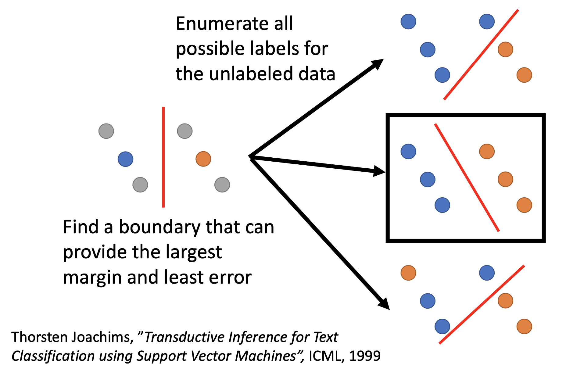
Semi-Supervised SVM
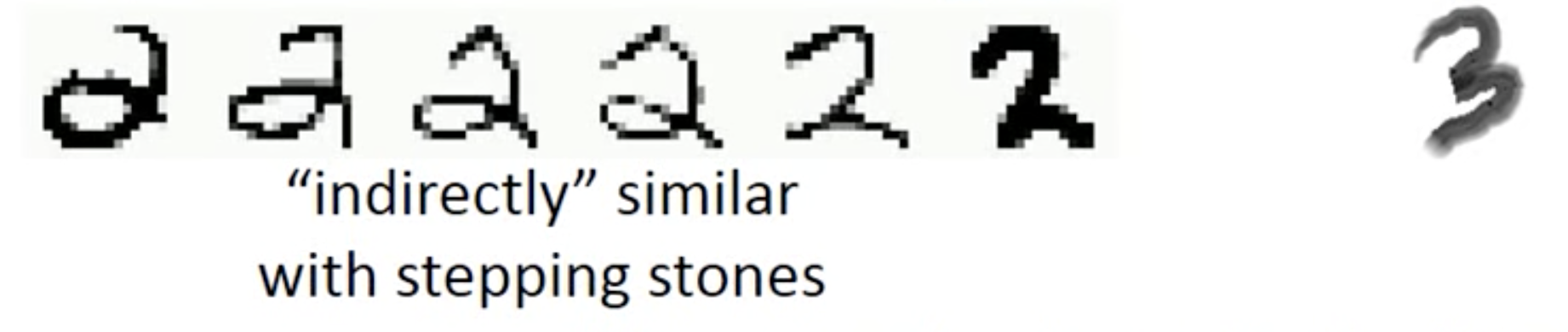
Smoothness Assumption
近朱者赤,近墨者黑。”You are known by the company you keep.”
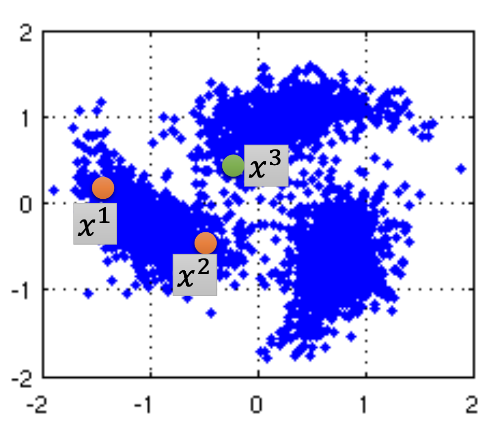
We assume similar $x$ has the same $\hat{y}$. To be precise, we assume:
- $x$ is not uniform.
- If $x^1$ and $x^2$ are close in a high density region, $\hat{y}^1$ and $\hat{y}^2$ are the same, i.e. $x^1$ and $x^2$ are connected by a high density path.
Cluster and Label
Make clustering first and then use all the data to learn a classifier as usual. In many cases, we has to use deep auto-encoder first to extract the feature to have good results.
Graph-Based Approach
Represent the data points as a graph to know the closeness / similarity between the data points so that we can define the high density regions and find the points connected by a high density path.
Graph representation is nature sometimes, e.g. Hyperlink of webpages, citation of papers. Sometimes we have to construct the graph ourselves.
Steps
Step 1: Define the similarity.
Define the similarity $s(x^i, x^j)$. For example, the Gaussian Radial Basis Function
\[s(x^i, x^j) = exp(- \gamma \vert \vert x^i - x^j \vert \vert ^2)\]is good for its fast decay.
Step 2: Add edges.
We can use the methods like K Nearest Neighbor or e-Neighborhood.
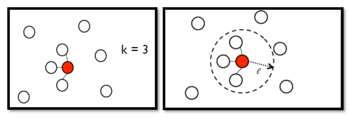
In this step, we need enough data points, or the graph may just break.
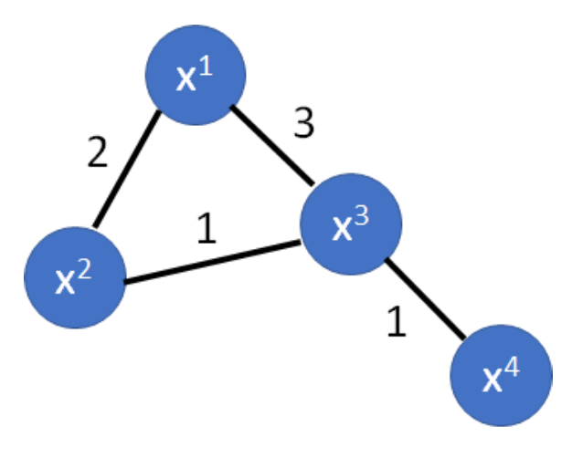
Step 3: Calculate weights on the edges.
Edge weight $w$ is proportional to $s(x^i, x^j)$.
Step 4: Minimize the loss function with the regularization based on smoothmess.
\[L = \sum_{x^r} C(x^r, \hat{y}^r) + \lambda S\]where S is the total smoothness.
Step 4 for Binary Classification
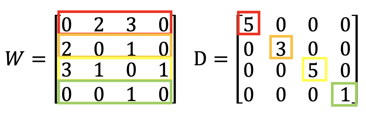
\[S = \frac{1}{2} \sum_{i \neq j} w_{i,j} (y^i - y^j)^2 = y^T L y\]where $y^i$ is between 0 & 1, and 0 & 1 represent the the 2 classes respectively. $y$ is a $R+U$-dim vector
\[y = \begin{bmatrix} \vdots \\ y_i \\ \vdots \\ y_j \\ \vdots \\ \end{bmatrix}\]and $L$ is the $(R+U)^2$ dimension matrix, the graph Laplacian, $L = D - W$. $W$ is the matrix of the off-diagonal $w_{i,j}$, $D$ is the diagonal matrix that each diagonal element is the sum of the off-diagonal elements at the same row.
Step 4 for More Classes
(My derivation)
\[S = \sum_{i \neq j}(1 - y^i \cdot y^j) w_{ij}\]where $y^i$ is a vector of the probability distribution, i.e. softmax output, to all the classes of example $i$. The inner product is the total probability that example $i$ and $j$ are in the same class, so the whole term is the weight times the probability that $i$ and $j$ are not in the same class.
Further discussion: By such definition of the smoothness, it seems that such definition lets all the unlabelled examples have a probability of 1 to a class and a probability 0 to all other classes, so there are no probability distributions anymore. I’m not sure whether such result is good and I should check it with some references.
Better Representation
去蕪存菁,化繁為簡。
Find the latent factors behind the observation, where the latent factors (usually simpler) are better representations.
My Discussion on Using the Methods simultaneously
How about perform self learning, entropy-based regularization and graph-based smoothness simultaneously?
It should be nonsense to use self learning and the others simultaneously because in self learning, we’re gradually include the unlabelled data into the labelled data. After that, there are no unlabelled data any more.
It should be ok to use entropy-based regularization and graph-based smoothness simultaneously. Entropy-based regularization tend to let all the unlabelled data get clear-cut rather than ambiguous classification, so it’s about the outputs from each unlabelled example itself and there are no direct mutual effects between examples. On the other hand, the smoothness approach handles the mutual effect between examples. The effects of entrophy-based regularization and smoothness approach are kind of indenpendent of each other, so it should be ok to use them simultaneously.