Notes for Prof. Hung-Yi Lee's ML Lecture 09: Tips for Deep Learning
Steps Toward a Successful DL Training
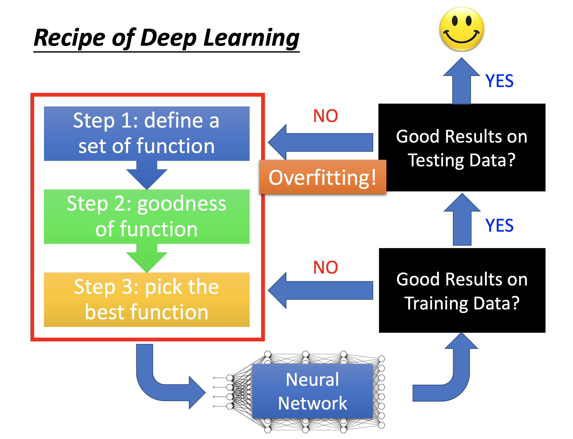
On many traditional ML models, e.g. decision tree or SVM, the performance on the training set is automatically 100% after training, so we don’t have to exam the model’s performance on the training set but just test the model on the testing set to see if it’s overgitting.
However, on DL, the training may just fail, so we have to exam the model’s performance on the training set to verify that the training is effective. After that, we can then test the model on the testing set to check if it’s overfitting. If the model fails on either the training or the testing set, we have to go back and check whether we have to do something different or apply some recipes in the 3 steps of ML.
With such charateristics, we can see that although DL models usually have much more parameters than traditional ML models, frequently overfitting is not the 1st problem we encounter in DL. Prior to overfitting, the training may just fails, and it’s even not so easy to produce overfitting.
Caution for Recognizing Overfitting
A model is overfitting only when a model performs well on the training set and performs poorly on testing set.
Scensrios and Their Recipes
For failure on training set, i.e. the training is not effective:
- New activation function.
- Adatative learning rate.
For failure on testing set, i.e. overfitting:
- Early stoping
- Regularization
- Dropout
Beware that for the recipes to improve performance on the testing set, here the testing set is the public testing set on kaggle or the validation set, for we don’t have the private testing set when we’re training models. My comments: the performace on private testing set should also be improved because we’re resolving over fitting.
New Activation Function
Vanishing Gradient
When using sigmoid function as the activation function on deep networks, vanishing gradient may occur because the sigmoid function compresses $0 \text{ to } \infty$ into $0 \text{ to } 1$. When it occurs, the gradient vanishes from the output end to the input end, the output end learns fast and the input end learn slowly. Consequently, when the output end already converges, the input end is still random. Also, because such convergence is based on the randomly initialized parameters, the performance is very poor.
In earlier days, peoplo resolve vanishing gradient by using RBM for initialization, freeze the output end and train the input end first, and then train the whole network.
Rectified Linear Unit (ReLu)
The relu function is
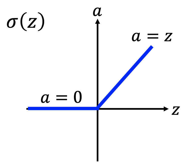
and $\frac{d \sigma}{dz} = 1$ when $z \geq 0$, $\frac{d \sigma}{dz} = 0$ when $z < 0$.
Reasons to use ReLu:
- Fast; low computing cost.
- Biologically reasonable.
- Can be reproduced by the sum of infinite sigmoid functions with different biases.
- Can handle the vanishing gradient problem.
By the behaviors of ReLu, it output 0 when input < 0 and is linear when input $\geq 0$, so it’s just like remove the neurons that are off, and the remaining network is just linear, then there won’t be vanishing gradient.
Is such “linearity” a problem for that what we want from a NN model is its nonlinearity? No. It’s linear only in a small range of input. By larger inputs, some neurons are turned on/off from off/on and then the network exibit nonlinearity.
Variants of ReLu:
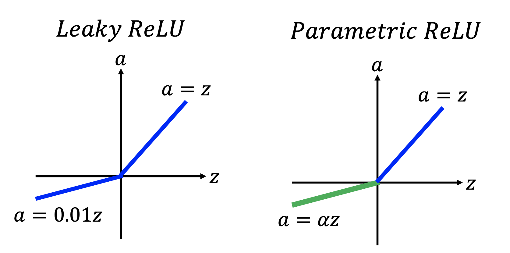
where in parametric Relu, $\alpha$ is also a parameter to be learned from training.
Maxout
Maxout is by grouping neurons and letting the groups pass only the maximum value in the group, for example
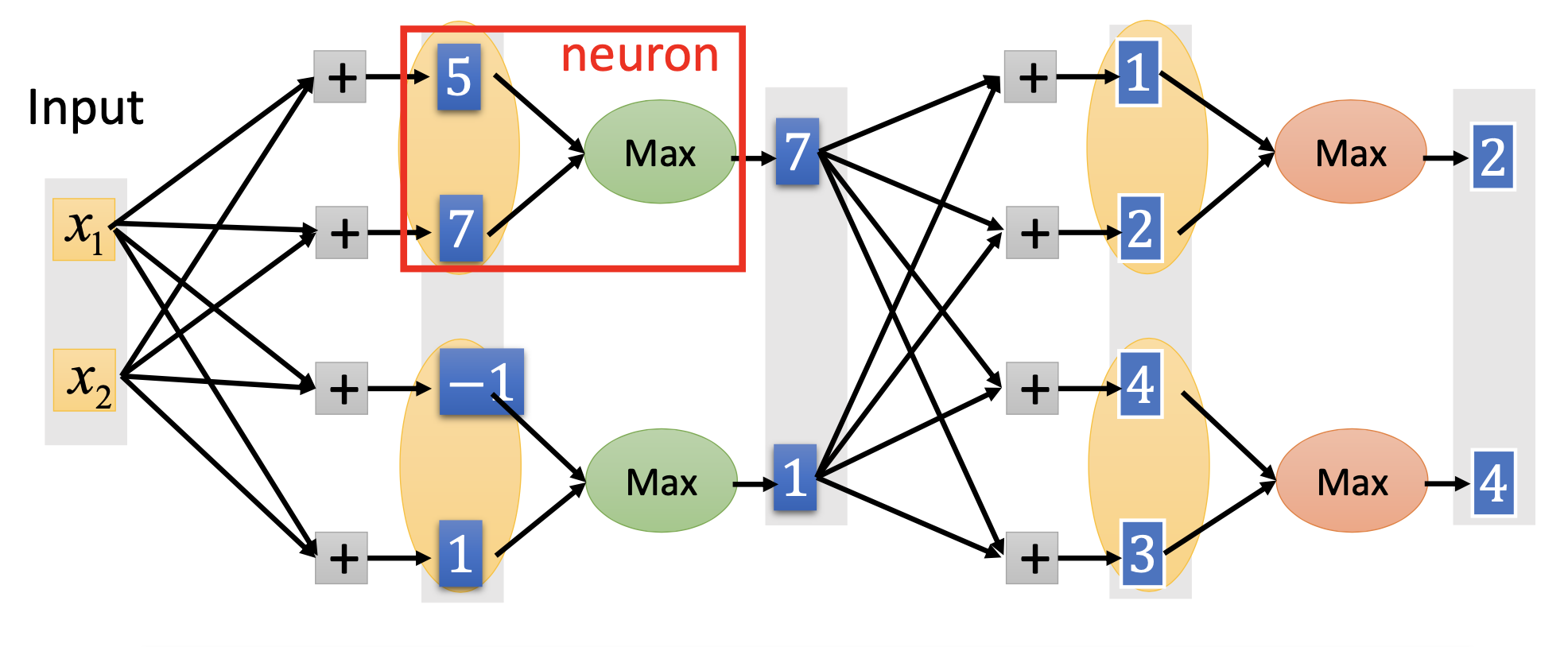
Maxout is a learnable activation function. The activation function in maxout network can be any piecewise linear convex functions, e.g.
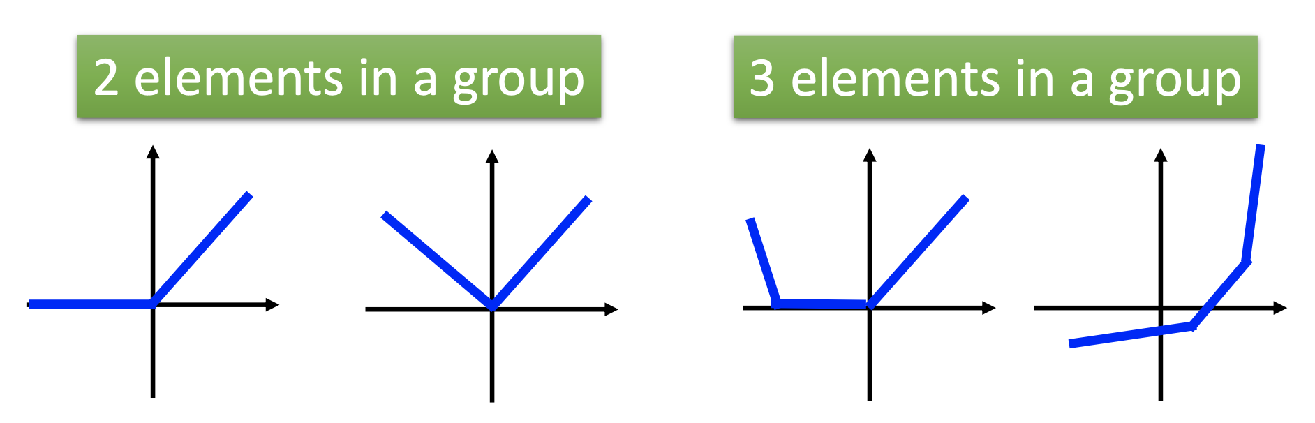
Also, ReLu is a special case of maxout.
Adaptive Learning Rates
In deep learning, the error surface may be complex, so wee need adaptive learning rates that can quickly adjust back and forth between high and low values. Adagrad cannot fulfill such need.
RMSProp
\[w^{t+1} \gets w^{t} - \frac{\eta}{\sigma^{t}} g^t\]where $g^t$ is gradient. $\sigma^0$ = $g^0$, $\sigma^t = \sqrt{\alpha (\sigma^{t-q})^2 + (1 - \alpha)(g^t)^2}$, so it’s the Root Mean Square of the gradients with decayed previous gradients.
Momentum
Let the updating of parameters has momentum like the real objects in the physical world:
\[v^{t+1} = \lambda v^t - \eta \nabla L(\theta^0)\]and move from $\theta^t$ to $\theta^{t+1} = v^{t+1} + \theta^t$. At the start, $v^0 = 0$. $v^t$ is actually the weighted sum of all the previous gradients.
On Local Minimum
Lecun: Don’t worry too much about stuck at local minimums. There are plenty of parameters in a network, and the chance is low to let all the derivatives of every parameter be 0, so there’re actually not so many local minimums.
Adam
Adam = RMSProp + Momentum.
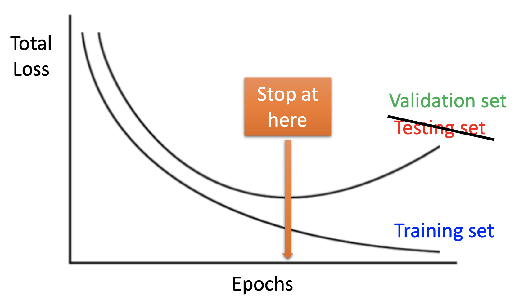
Early Stoping
Stop the training before the network start to be overfitting. Beware that the public testing set may be too small, so use we should stop training based on the validation set.
Regularization
By regularization, we minize a new loss function $L’$ such that the weights not only minimize original loss but also are close to zero, i.e. smoother.
L2 Regularization
\[L'(\theta) = L(\theta) + \lambda \frac{1}{2} \vert \vert \theta \vert \vert_2\]where the L2 norm $\vert \vert \theta \vert \vert_2 = \sum_j (w_j)^2$. Then we update the $w$ by
\[w^{t+1} \gets (1 - \eta \lambda)w^t - \eta \frac{\partial L}{\partial w}\]and we can see the weights decay by updaes.
L1 Regularization
\[L'(\theta) = L(\theta) + \lambda \vert \vert \theta \vert \vert_1\]where the L1 norm $\vert \vert \theta \vert \vert_1 = \sum_j\vert w_j \vert$. Then we update the $w$ by
\[w^{t+1} = w^t - \eta \lambda sgn(w^t) - \eta \frac{\partial L}{\partial w}\]and we can see the updates constantly delete the weights.
Comparing L1 & L2 Regularization
By the different characteristics of L1 & L2 regularization, they are suitable for different scenarios.
| For Large $w$’s | For small $w$’s | Overall effect | |
|---|---|---|---|
| L1 | No strong decay => keep the big values. | Fixed deletion => near 0. | Sparse |
| L2 | Strong decay => no big values. | Small decay => keep the small values. | Dense |
Comparing with Regularization in Traditional ML Models
Unlike in some traditional ML models, e.g. SVM, the effectiveness of regularization is not very significant in DL. A possible reason is that all the weights start from values near 0 in the beginning, so the effect of regulatization is actually similar to early stopping.
Dropout
In training, in each mini-batch, we resample the neurons, i.e. drop some neurons out, by a rate p%.
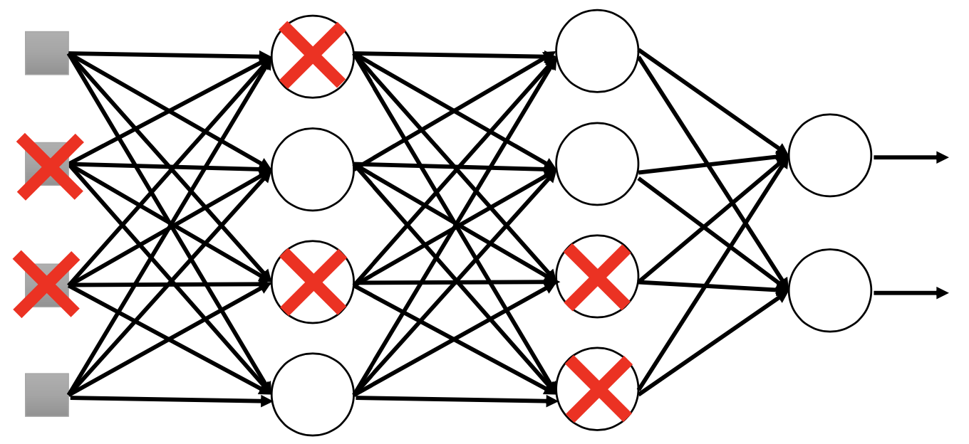
And in testing, we multiply all the weights by 1 - p% and use the whole network to inference.
Dropout is a kind of ensemble: it’s like to train many slighly different networks that shares their weights, and then use the average of all the networks’ outputs are the final output. The average effect can then reduce the variance from the complex model.
Using dropout with ReLu performs better than with sigmoid. The reason may by that ReLu is closer to linear function, and by linear functions the average of the dropout networks and the output of the 1 - p% final network are identical.
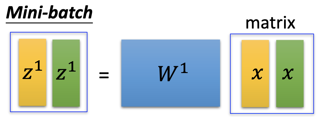
Mini-Batch Size, Training Speed & GPU
In DL, we actually don’t minimize total loss but only the loss on mini batches. Computing gradients by all the examples may take too large memory spaces. Also, if we don’t use mini-batches for optimization, the total number of steps of updates may be too low to find the local minumum, or the gradients may align too perfectly on the normal to have randomness to get out of the local minimums.
On the other hand, the mini-batch sizes have to be big enough so that we can benefits from GPU to boost the training. As shown in the figure below, the computing time for a minibatch is actually the same as for a single example.
References
Youtube ML Lecture 9-1: Tips for Training DNN
For Mini-Batch Size, Training Speed & GPU