Notes for Prof. Hung-Yi Lee's ML Lecture 5, Classification: Logistic Regression.
Logistic Regression
The 1st step of ML, choosing the function set:
If $P(C_1 \vert x) \geq 0.5$, Output $C_1$; Otherwise, Output $C_2$. where
\[P(C_1 \vert x) = \sigma(z) \text{, } z = w \cdot x + b \text{, } \sigma(z) = \frac{1}{1 + e^{-z}}\]The 2nd step of ML, goodness of functions:
The likelihood to get the training examples is
\[L(w, b) = \prod_{x^k \in C_1} f_{w,b}(x^k) \prod_{x^k \in C_2} (1 - f_{w,b}(x^k))\]and then maximize the likelihood by
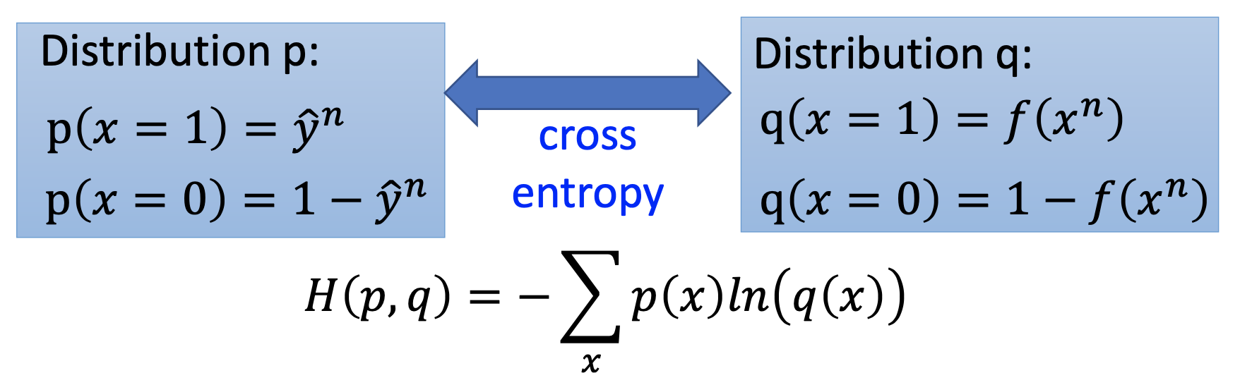
\[w^*, b^* = arg \max\limits_{w, b}L(w, b) = arg \min\limits_{w, b} -lnL(w,b)\] \[-lnL(w, b) = - \sum_{n}[\hat{y}^n ln f_{w,b}(x^n)+ (1 - \hat{y}^n) ln(1 - f_{w,b}(x^n))] \\ = \sum_{n} C( \hat{y}^n, f(x^n) )\]where C is cross entropy.
The 3rd step of ML, find the best function
By gradient descent, we calculate $\frac{\partial (-lnL(w,b))}{\partial w_i}$ and $\frac{\partial (-lnL(w,b))}{\partial b}$, then we update $w$ and $b$ by
\[w_i \gets w_i - \eta \sum_{n} - (\hat{y}^n - f_{w,b}(x^n)) x_i^n\] \[b \gets b - \eta \sum_{n} - (\hat{y}^n - f_{w,b}(x^n))\]Logistic Regression v.s. Linear Regression
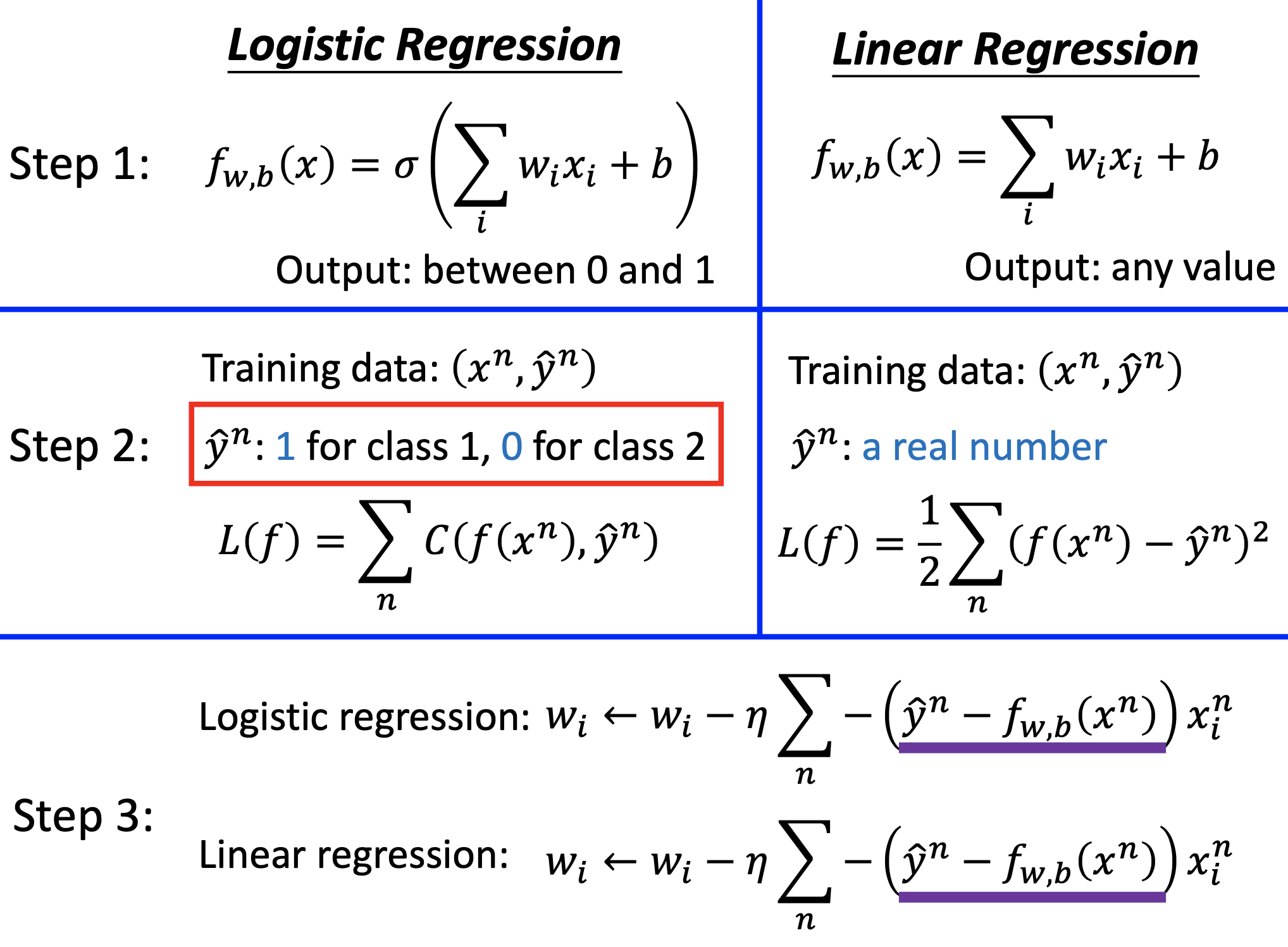
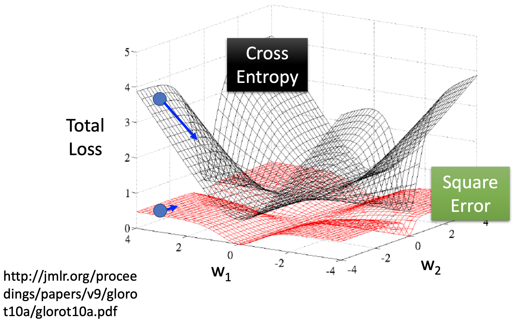
Why not use rms error on logistic regression?
In step 3,
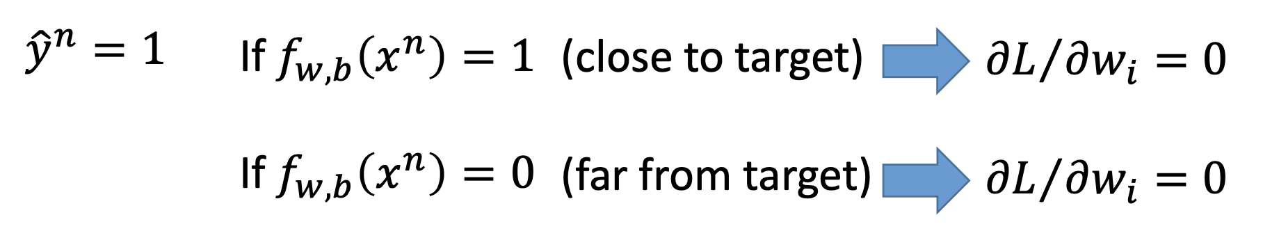
\[\frac{\partial (f_{w,b}(x)- \hat{y}^n)^2}{\partial w_i} = 2(f_{w,b}(x^n)- \hat{y}^n)f_{w,b}(x^n)(1-f_{w,b}(x^n))x_i^n\]then
Generative vs Discriminative
For $P(C_1 \vert x) = \sigma(w \cdot x + b)$, by generative model, we find $\mu^1$, $\mu^2$ and $\Sigma^{-1}$, then we calculate $w$ and $b$ by the 3 parameters; while by discriminative, we find $w$ and $b$ directly. We may (highly possibly) obtain different $w$ and $b$ by the 2 approaches.
By Prof. Lee’s comment, with different approaches, we may get different the best functions from the same function set. However, by my understanding, the 2 different approaches are actually defining differnt function sets. Due to the constraints by the statistical distribution, the generative approach has a smaller function set.
In conclusion, the discriminitive modeld may have better performance whezn given enough training examples.
On the other hand, with the assumption of probability distribution, the generative modeld needs less traning examples, are more robust to noises, and the priors and class-dependent probabilities can be estimated from different sources. For example, in speech recognition, we can train the generative model by texts to build probabilistic models, so that we can reduce the amount of voice data required.
Try to compare the size of function sets by degrees of freedom
By the discussio below, I intended to show that the size of the function set of discrimitive model is larger than the generative model, but I failed.
By the generative approach, the training examples and the gaussian distribution yields exactly 1 set of the 3 parameters $\mu^1$, $\mu^2$ and $\Sigma^{-1}$. When a feature of the input or the output of an example changes, all the 3 parameters follow the changes simultaneously, so the degree of freedom is the number of dimentions of input + 1.
On the other hand, by the discriminative approach, by choosing different learning rate or methodology of gradient descent, all the dimensions of $w$ and $b$ may change independently. so the degree of freesom is the number of dimentions of input + 1.
Multiclass Logistica Regression
The 1st step of ML, choosing the function set:
$y_i = P(C_i \vert x)$, where $1 > y_i > 0$ and $\sum_i =1$, and
\[y_i = \frac{e^{z_i}}{\sum_{j=1}^{N_c} e^{z_j}}\]is the softmax function, where $z_i = w^i \cdot x + b_i$, $N_c$ is the tot number of classes.
The 2nd step of ML, goodness of functions:
We use the cross entrooy
\[- \sum_{j = 1}^{N_c} \hat{y}_j ln y_j\]The 3rd step of ML, find the best function
We use gradient descent
\[w_j \gets w_j - \eta \sum_{n=1}^{N_{tot}} (y_{nj} - \hat{y}_{nj}) x_n\]Limitations of Logistic Regression
The boundary between classes is linear, to logistic regressions can’t learn to classify some examples like
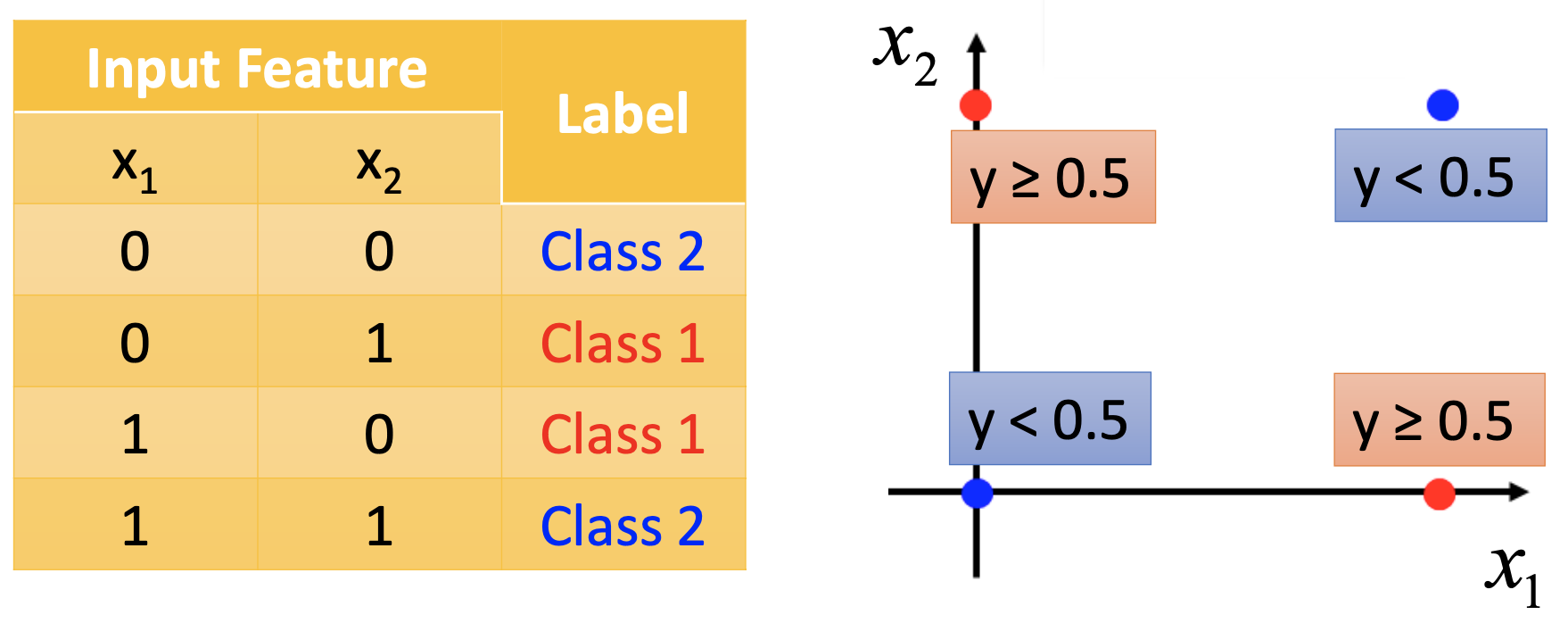
for such examples, we can perform feature transformation 1st and then use logistic regression, e.g.
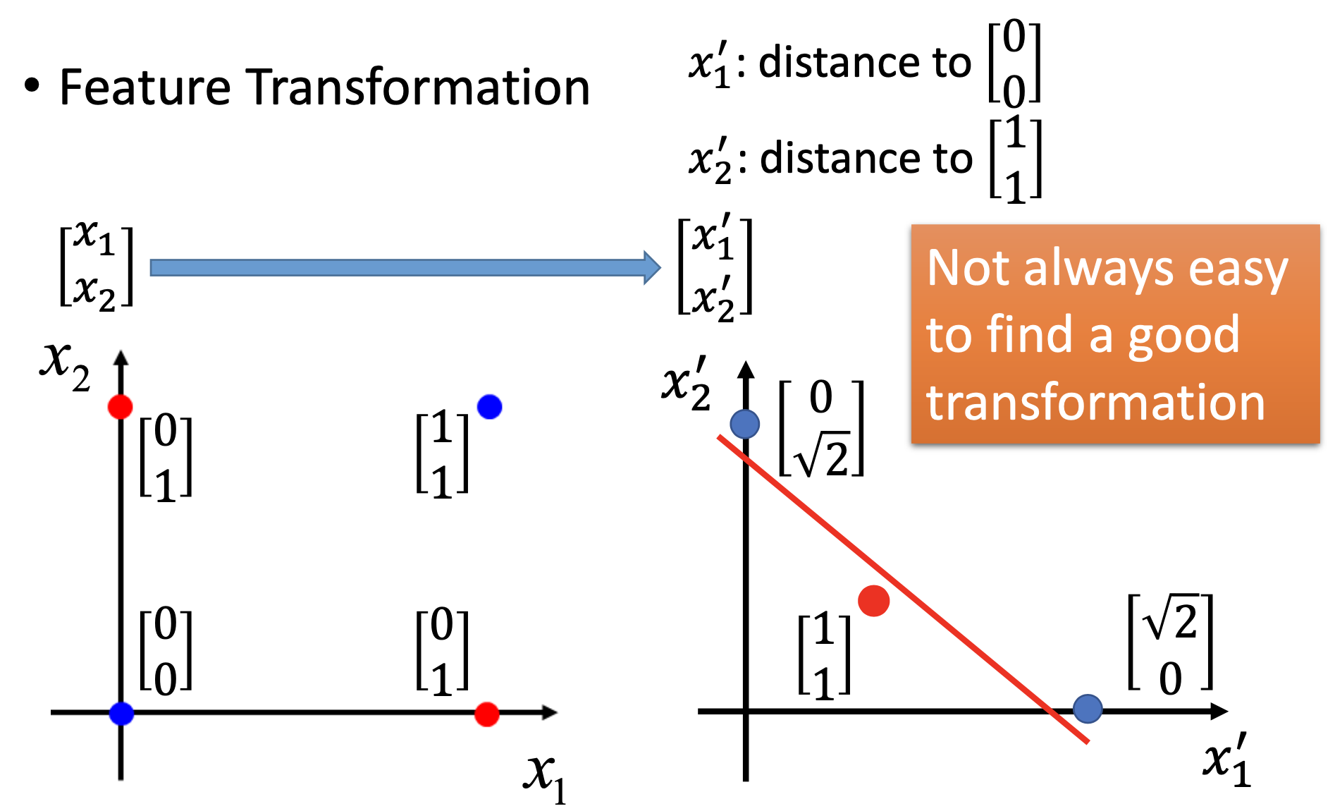
however, it’s not always easy for us to find how to perform the feature transformation effectively. If we choose the cascaded logistic regression as the model and train it, we are actually using the neural network.
References
Youtube ML Lecture 5: Logistic Regression
<Pattern Recognition and Machine Learning>, Christopher M. Bishop