Notes for Prof. Hung-Yi Lee's ML Lecture 4, Classification: Probabilistic Generative Model.
What are Classification Problems
Input features & output the class that the input should belong to.

The effectiveness of Solving Classification as Regression
If we use value 1, 2, 3, 4 … as the outputs of classes, there may be problems. 1st, there may be penalty to the examples that are “too correct”. For example:
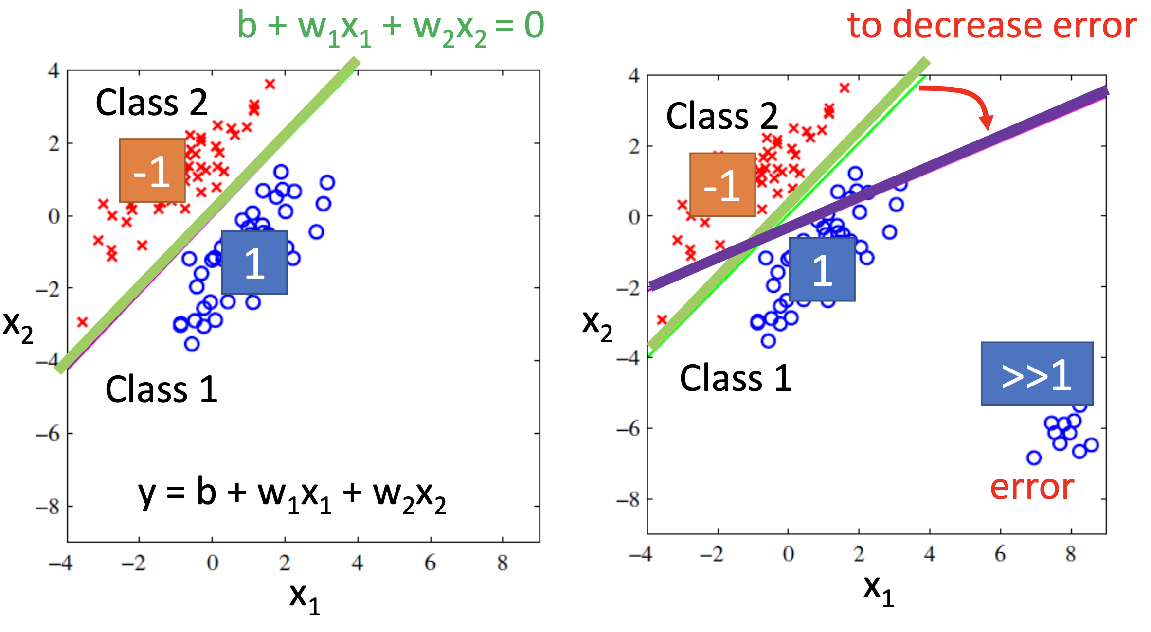
2nd, such approach implicitly assumes that the neighboring classes (e.g. 1 & 2, 5 & 6) are quantitative closer than other classes, which is false by the meaning of “classes”.
Ideal approaches to classification
Probabilistic Generative Model
Generative: we can use the trained model to generate new examples.
Here we consider a binary classification problem.
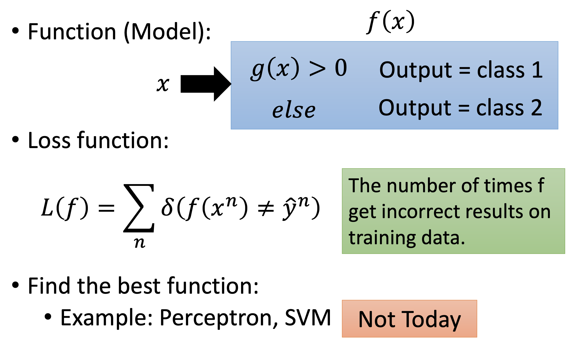
The 1st step of ML, choosing the function set:
given an example $x$, if $P(C_1 \vert x) > 0.5$, i.e. the probability that this example is from class $C_1$ > 0.5, then output $C_1$, otherwise output $C_2$. By probability,
\[P(C_1 \vert x) = \frac{P(x \vert C_1)P(C_1)}{P(x \vert C_1)P(C_1) + P(x \vert C_2)P(C_2)}\]$P(C_i)$ is the probability that an example is from class $C_i$. so
\[P(C_i) = \frac{N_i}{N_1 + N_2}\]where $N_i$ is the total count of examples of class $C_i$.
For $P(x \vert C_i)$, let’s assume Gaussian distribution
\[f_{\mu , \Sigma}(x) = \frac{1}{(2 \pi)^{\frac{D}{2}} \vert \Sigma \vert^{\frac{1}{2}}} e^{- \frac{1}{2}(x - \mu)^T \Sigma^{-1} (x - \mu)}\]where $\mu$ is mean and $\Sigma$ is covariance matrix.
Besides, the generative model $P(x) = P(x \vert C_1)P(C_1) + P(x \vert C_2)P(C_2) $
The 2nd step of ML, goodness of functions:
Let’s maximize the likelihood $L(\mu_i,\Sigma_i)$, the probability to generate all the training examples of class $C_i$:
\[L(\mu^i,\Sigma^i) = \prod_{x^k \in C_i} f_{\mu^i , \Sigma^i}(x^k)\] \[\mu^{i*} , \Sigma^{i*} = arg \max\limits_{\mu^i , \Sigma^i}L(\mu^i,\Sigma^i)\]The 3rd step of ML, find the best function
then we know
\[\mu^{i*} = \frac{1}{N_i} \sum_{x^k \in C_i} x^k\] \[\Sigma^{i*} = \frac{1}{N_i} \sum_{x^k \in C_i} (x^k - \mu^{i*})(x^k - \mu^{i*})^T\]Gaussian Model to Logistic Regression
In the demo, the former model doesn’t perform well due to overfitting. When there are $N_f$ features, if we that the 2 classes have different covariance matrices, there’ll be $2N_f^2$ parameters. If we let the 2 classes share the same covariance matrix, the performance can be improved.
After sharing the same covariance matrix, $\mu^1$ and $\mu^2$ is the same as before, and the new $\Sigma$
\[\Sigma = \frac{N_1}{ \frac{N_1}{N_{tot}} \Sigma^1 + \frac{N_2}{N_{tot}} \Sigma^2}\]Posterior Probability
Definition of posterior probability: the probability of the parameters $\theta$ given the evidence $X$, $p(\theta \vert X)$; the probability of the class $C$ given the example $x$, $p(C \vert x)$.
To calculate the posterior probability, let
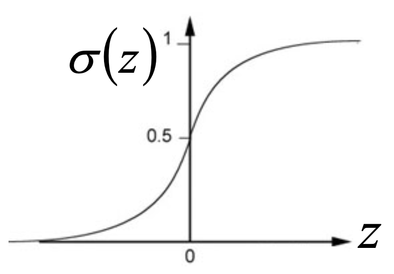
\[P(C_1 \vert x) = \frac{P(x \vert C_1)P(C_1)}{P(x \vert C_1)P(C_1) + P(x \vert C_2)P(C_2)} \\ = \frac{1}{1 + e^{-z}} = \sigma(z)\] \[z = ln \frac{P(x \vert C_1)P(C_1)}{P(x \vert C_2)P(C_2)}\]where $\sigma$ is the sigmoid function.
and then
\[P(C_1 \vert x) = \sigma(w \cdot x + b)\]where
\[w^T = (\mu^1 - \mu^2)^T\Sigma^{-1} \\ b = - \frac{1}{2} (\mu^1)^T \Sigma^{-1} \mu^1 + \frac{1}{2} (\mu^2)^T \Sigma^{-1} \mu^2 + ln \frac{N_1}{N_2}\]In generative model, we estimate $\mu1$, $\mu2$ and $\Sigma$, then we get $w$ and $b$. If we find $w$ and $b$ directly, such method is logistic regression.
More than 2 classes
When there are more than 2 classes,
\[P(C_1 \vert x) = \frac{1}{1 + \sum_{k \neq 1} \sigma(w^{k} \cdot x + b^k)}\]where
\[(w^k)^T = (\mu^1 - \mu^k)^T\Sigma^{-1} \\ b^k = - \frac{1}{2} (\mu^1)^T \Sigma^{-1} \mu^1 + \frac{1}{2} (\mu^k)^T \Sigma^{-1} \mu^k + ln \frac{N_1}{N_k}\]then it’s not logistic regression.
Choosing the distribution
Choose whatever the distribution you like, e.g. for binary features, it may be reasonable to choose Bernoulli distribution. Or if we assume all dimensions are independent, then it becomes the Naive Bayes classifier.