Notes for Prof. Hung-Yi Lee's ML Lecture 3, gradient descent.
Vanilla Gradient Descent Formulation
For a loss function $L(w)$:
- (Randomly) pick initial $w^0$.
- $w^1 \gets w^0 - \eta \nabla L \vert_{w=w^0}$, where $\eta$ is the learning rate.
- repeat step 2 to get $w^2$ … $w^T$ after $T$ iterations.
Finally, we can get a local minimum (possibly the global minum).
Gradient Descent Tip 1: Tuning Learning Rate
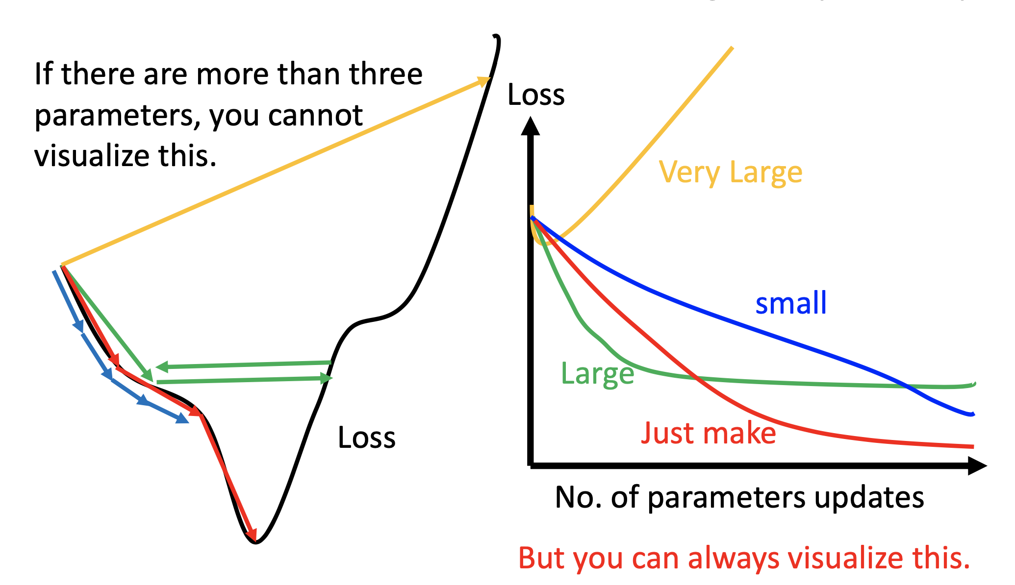
Loss to # of Updates Plots
Always plot loss to # of updates to check the performance of the chosen learning rate.
Adaptive Learning Rates
Reduce Learning Rate by Epochs
At the beginning, we are far from the destination, so we use larger learning rate. After several epochs, we are close to the destination, so we reduce the learning rate. For example: $ \eta^t = 1 / \sqrt{1 + t}$.
Use Different Rate for Different Parameters
Learning rate cannot be one-size-fits-all, so give different parameters different learning rates.
Adagrad
Divide the learning rate of each parameter by the root mean square of its previous derivatives.
\[w^{t+1}_{j} \gets w^{t}_{j} - \frac{\eta^t}{\sigma^t_j} g^t_j\]where $ w^{t}_{j} $ is the $j$th parameter at the $t$th iteration,
$ \eta^t = 1 / \sqrt{1 + t} $, $ g^t = \frac{\partial L(w^t)}{\partial w^t_j} $ and $ \sigma^t_j = \sqrt{\frac{1}{t+1} \sum_{k=0}^{t}\vert g^k \vert^2} $. then
\[w^{t+1}_{j} \gets w^{t+1}_{j} - \frac{\eta}{\sqrt{\sum_{k=0}^{t} \vert g^k \vert^2}} g^t_j\]Due to the denominator, the stepping speed get slow at large step counts. Adam don’t have such problem, and Adam may be currently the most stable choice.
Discussion on the Relation between Step Size and Gradient
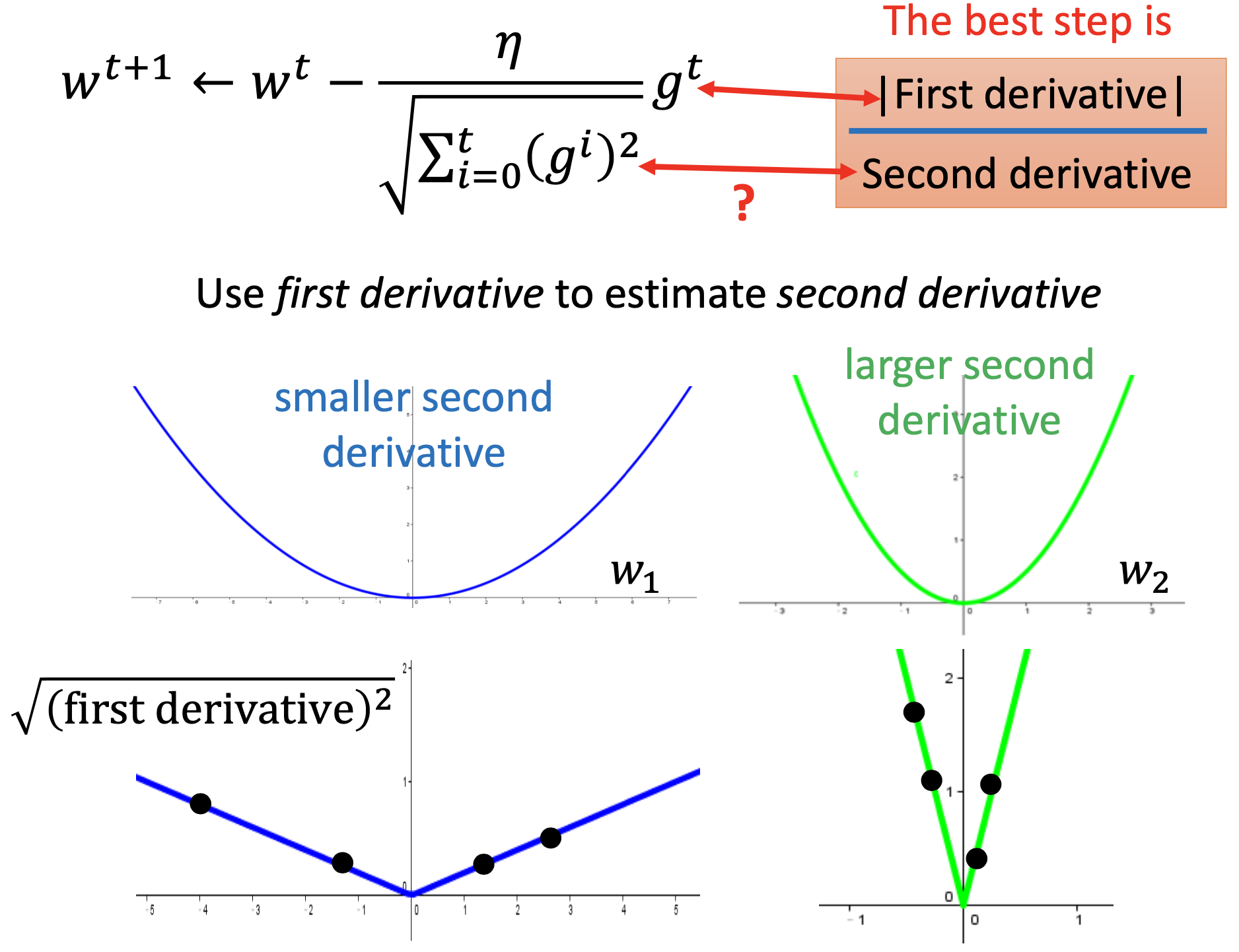
By $g^t_j$, larger gradient lead to larger step, while by $\sqrt{\sum_{k=0}^{t} \vert g^k \vert^2}$, larger gradient lead to smaller step. Is there any contradiction?
The intuitive reason: the denominator can serve as a measure of supprise. (My comment: it’s true only when the gradient suddenly goes smaller. When a gradient suddenly goes larger, the new gradient dominate in the denominator, and then the denominator cancels with the numerator, so the new step size is similar to the previous ones.)
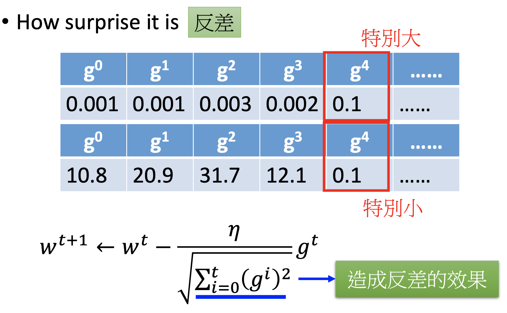
The formal explanation: “the larger the gradient, the larger the step size” is incorrect in the context of multi-parameters.
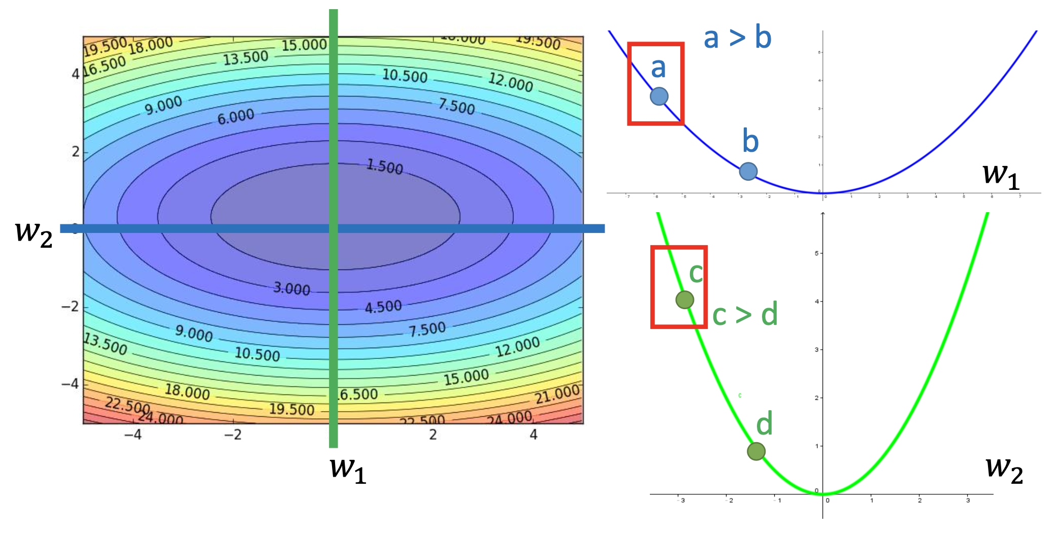
Also, by $y = a x^2 + bx + c$, we know that the best step from $x_0$ is $\frac{\vert 2ax_0 + b \vert}{2a}$, where $2a$ is the 2nd derivative.
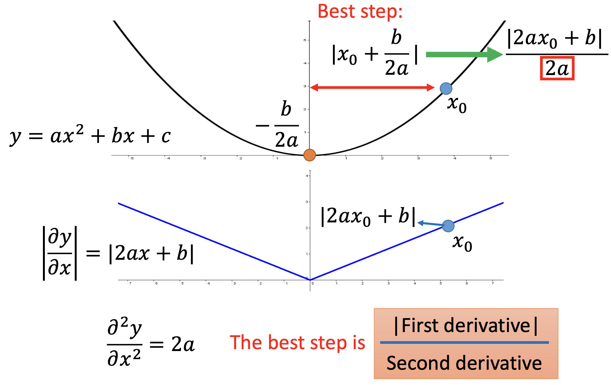
To avoid the computing cost of the 2nd derivatives, we use 1st derivatives to estimate the 2nd derivatives.
Gradient Descent Tip 2: Stochastic Gradient Descent
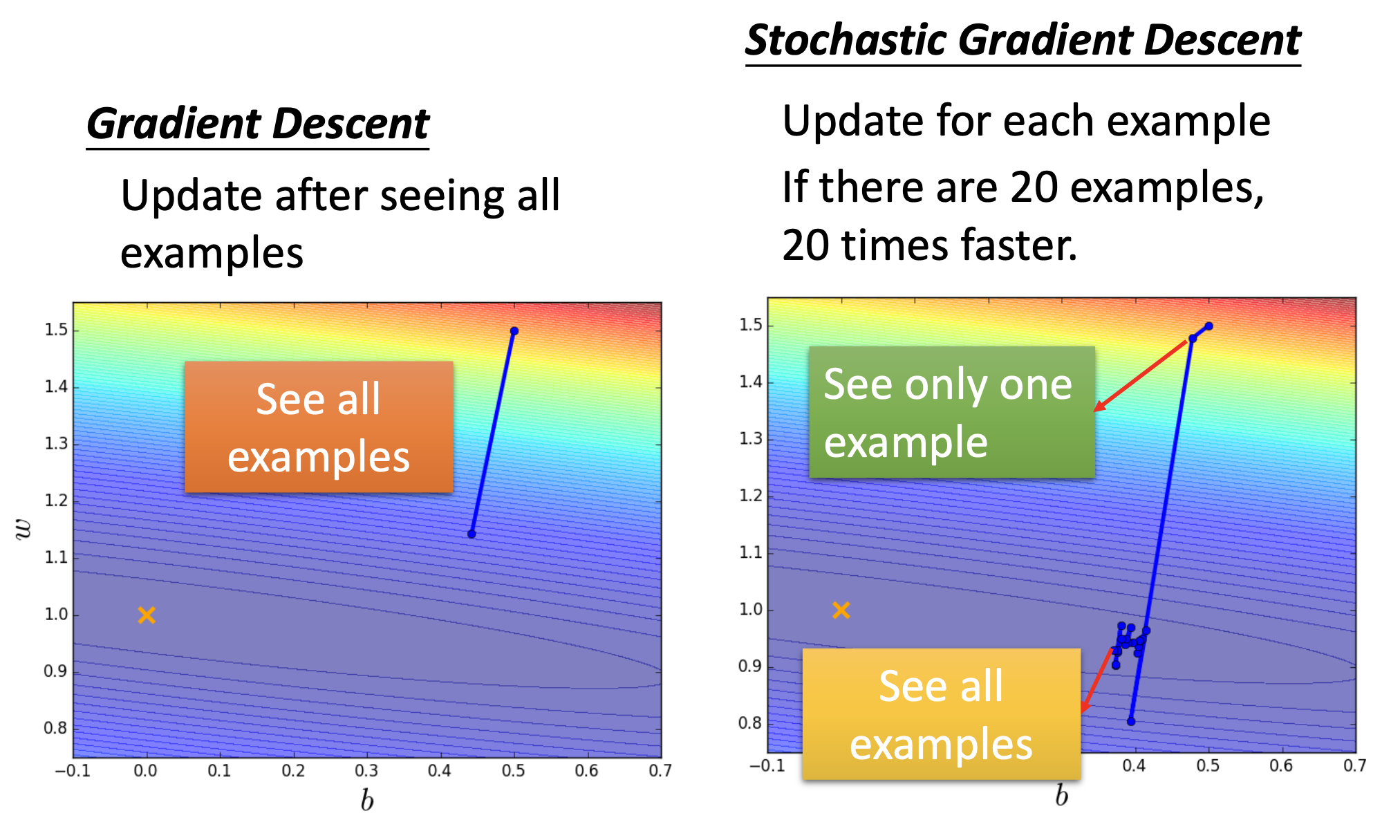
In vanilla gradient descent, the loss is computed by the summation over all training examples. In stochastic gradient descent, for every step, the loss is computed by onlt 1 training example. Such change can make the training faster because there are N times more steps.
Gradient Descent Tip 3: Feature Scaling
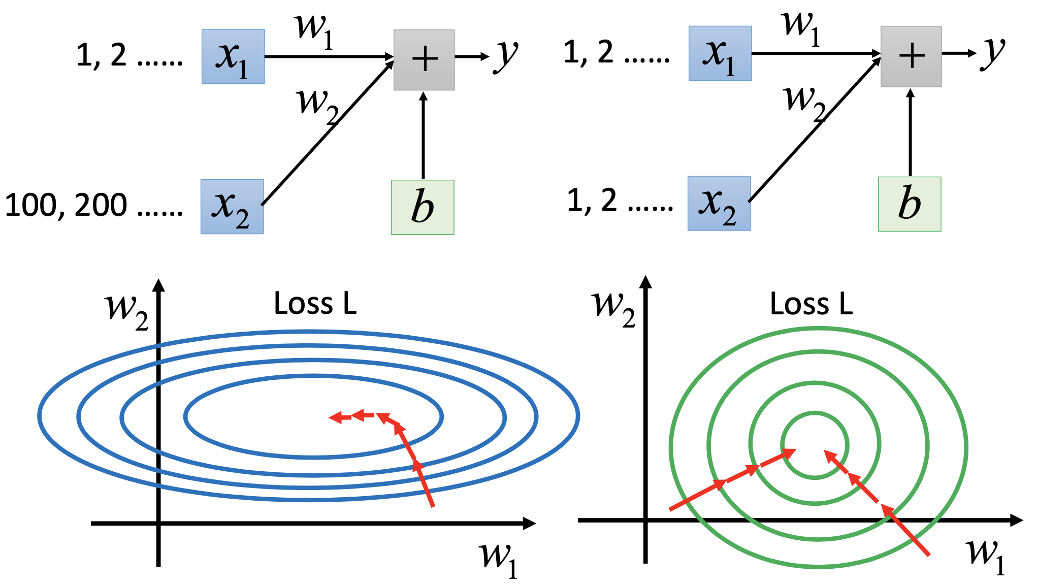
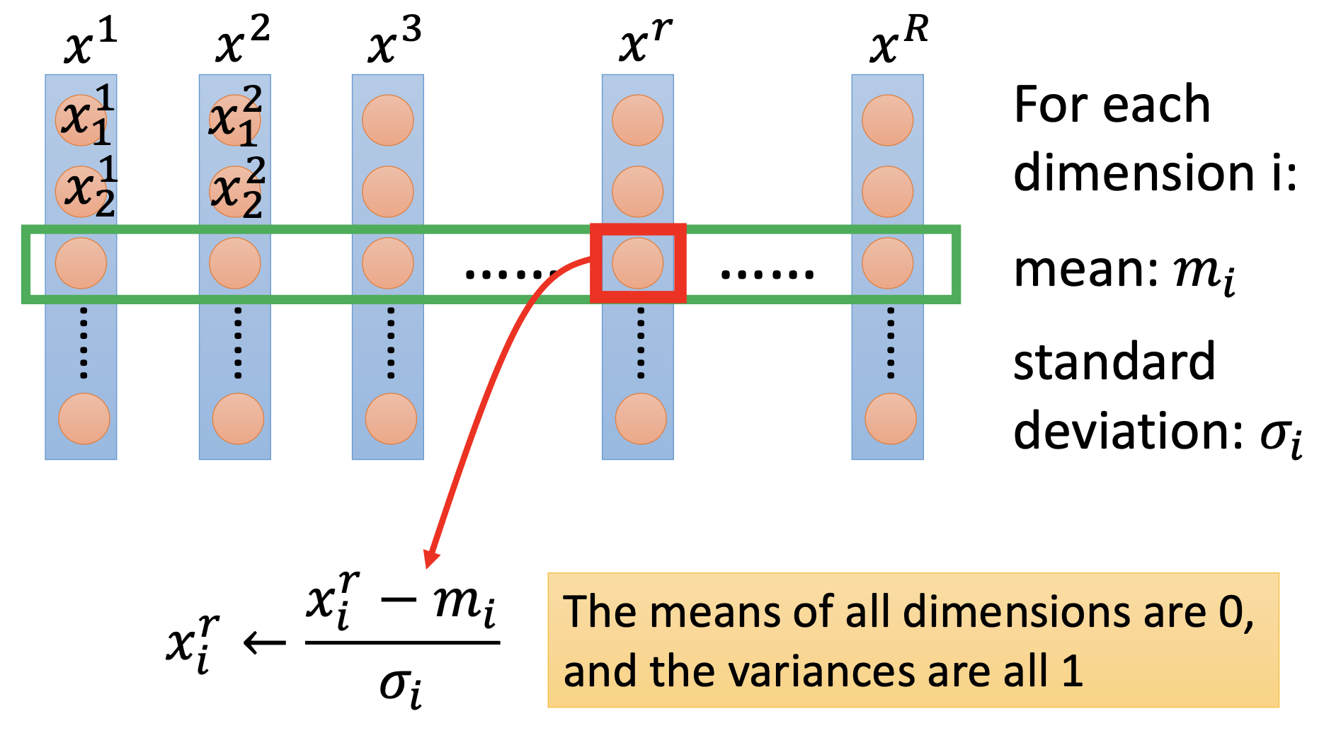
By centering and normalizing the input features, the minimum will be on the direction of the gradient, thus lead to easier optimization.
Proof for the Correctness of Gradient Descent
In a small sphere near $w^0$, we find the position with the lowerest loss as $w^1$. By contineuing this process, we can find the local minimum.
By Taylor’s theorem, if the sphere is small enough, then the minimum in the sphere is on the line $ w^0 - \eta \nabla L \vert_{w=w^0}$, where $\eta$ is a positive number.
In conclusion, theoretically, gradient descent can get the local minimum only when the step size is small enough.
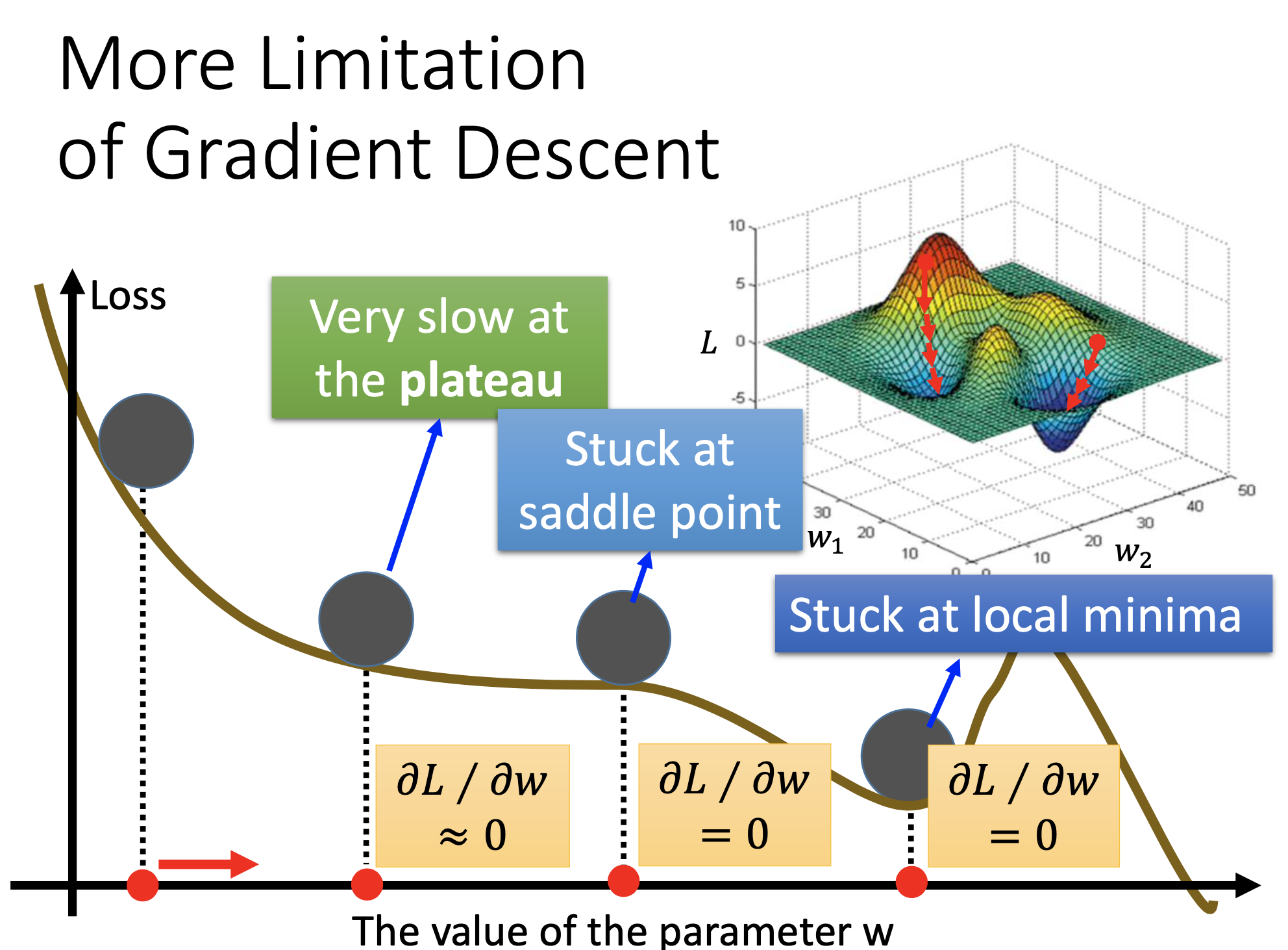
More Limitaions of Gradient Descent
References
Youtube ML Lecture 3-1: Gradient Descent
Youtube ML Lecture 3-2: Gradient Descent (Demo by AOE)
Youtube ML Lecture 3-3: Gradient Descent (Demo by Minecraft)